Geometry and set up the steady problem of horizontal axis wind turbine (hawt)

 

To study of the flow around the wind turbine via Computational Fluid Dynamics (CFD) software, firstly it is need to construct themodel of the object and to mesh the considered domain of the object. It requires to be familiarized with the concepts on functioning of the Horizontal Axis Wind Turbine (HAWT) and of course, the knowledge on Discretization theory and Finite elements. Here, we also review the appropriate turbulence model for simulation in order to describe the turbulent flow region around the wind turbine.

Key words: wind turbine, nacelle, blades, grid, meshing techniques, turbulence, Navier-Stocks equations.

Исследование обтекания ветровой турбины с помощью программного обеспечения «ComputationalFluidDynamics» (CFD) показали: во-первых, это необходимо, чтобы построить модель объекта и сетки рассматриваемой области объекта. Для решения этой проблемы необходимо изучать основные понятии функционировании ветряных турбин с горизонтальной осью, и конечно, знание теории дискретизации и применения методов конечных элементов. Для изучения турбулентности вокруг ветровой турбины рассмотрим соответствующую модель турбулентности.

Ключевые слова: ветровая турбина, гондола, лопасть, сетки, сеточные методы, турбулентность, уравнение Навье-Стокса.

 

1.Introduction. A wind turbine is a device for extracting kinetic energy from the wind. By removing some of its kinetic energy the wind must slow down but only that mass of air which passes through the rotor disc is affected. So behind the rotor disc the nacelle wind speed differs from the free stream wind speed . For managing and optimizing the wind farm power production an accurate calculation of nacelle wind speed is demanded. But, when we begin to study the wind turbine and its power productions we face firstly to the design and geometry of the wind turbine.

This work is focused on using software Gambit for presenting the geometry of the Horizontal Axis Wind Turbine (HAWT), realization of mesh generation as well as choice of the appropriate turbulence model that would be implemented in the simulation of airflow using CFD software in order to study of the flow behavior around and within a rotating wind turbine.

The large increasing penetration of large wind turbines into electrical power systems is inspiring continuously the designers to develop both custom genera­tors and power electronics, and to implement modern control system strategies. In addition to becoming larger, wind turbine design con­cepts have been progressing from fixed speed, stall-controlled and drive trains with gearbox to variable speed, pitch controlled with or without gearbox [1, 3].

2. Geometry and set up the steady problem of HAWT. The horizontal axis wind turbine has a three blade rotor with radius of 40 m and hub radius of 1.696 m. The blades are rectangular tip blades. They have a chord of 0.48 m at tip and 3.52 m at the root. The rotational speed is 2.8 rad/sec with a free stream velocity of 16 m/s. Hence, the TSR (tip speed ratio) is equal to 7. To investigate the flow field around the horizontal axis wind turbine, in the simulation we consider that the rotational periodicity is not used and a flow past the rotor is modeled completely and not only one period. The periodicity is not used because this improves the unsteady simulation. In order to model the flow blockage the rotor is modeled as it rotates in the wind tunnel. Therefore the tunnel walls are modeled to confine the flow about the rotor and this creates more realistic induced velocities.

The sliding mesh technique is used in the simulation because, as we are looking through the rotating case it gives an opportunity to use the changing variables in the resolution of Navier Stokes equations in such a way that we do not need to do mesh for each movement of the rotor. Hence, the flow field is divided into two distinct cell zones; one is a parallelepiped that represents the wind tunnel and the other one that represents the turbine rotor is a cylinder.

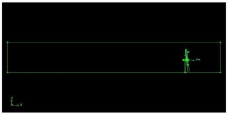
Figure 1: Parallelepiped and cylinder zones

The cylinder, which includes the blades, has diameter 1.05D and length 0.06D. Here D = 80 m is the diameter of the rotor. The computational domain is a parallelepiped of dimensions 650 x 150 x 120 which is extended about 6.8 diameters of the rotor downstream and 1.25 diameters of the rotor upstream in the axial direction.

Different size mesh generation has been presented taking into account the different range of geometric scales such that: length of the parallelepiped domain (650 m), size of rotor (40 m), height of the tower (48 m) and the diameter of the cylinder (84 m) (see Figure 1).

In order to take care of the local geometric scales, each zone is meshed using the journal file. The triangles and tetrahedral elements axe used for meshing and are scaled in m.

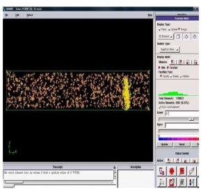
As the faces of blade tips are small, we have meshed there with an interval size of 0.1 m. On the suction and pressure surfaces of the blades firstly the edge meshes are generated with the double sided successive ratio 1.02 and interval size 0.5 m, because of small tip and root faces of the blades are then meshed automatically. In order not to obtain too many elements in the cylinder region, because of computational cost, we have used in that zone the meshed type size function, taking as the source faces the faces of blades and hub. The total number of elements in the cylinder volume is 745863 and the EquiSize Skew quality 0.7647. The grids of size 1 with the successive ratio 0.99 are used to generate the mesh on the edges of the tower. In order to have more elements behind the rotor, we created the meshed size function with the source faces including the tower surfaces and nacelle faces. Finally, the total number of computational cells amounts to 1.8 million with the poor EquiSize Skew quality 0.797828 [4], but it is not bad because it is not located in the region that should be cared. The mesh quality is poor [4] but the number of bad elements is reduced (see Figure 2).

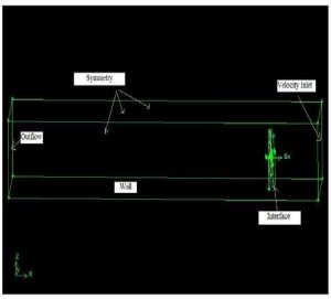
To export the mesh, the following types of boundary conditions are specified: velocity inlet, outflow, symmetry, wall and interface as indicated in the Figure 3, and the two existing volumes are specified as fluids.

Here we assume that all computations will be carry out in steady state condition.

Figure 2. The worst element around the turbine Figure 3.Boundary conditions

3. Choosing the appropriate turbulence model

We employ the Reynolds averaged Navier-Stokes (RANS) approach to our model because the RANS-based modeling approach greatly reduces the required computational effort and resources, and is widely adopted for practical engineering applications.

For steady and incompressible flow conditions around the turbine and nacelle, the time averaged continuity and the Navier-Stokes equations are written in Cartesian form as

(1)

(2)

Additional terms now appear that represent the effects of turbulence. These Reynolds stresses, must be modeled in order to close Equation (2).

The Reynolds-averaged approach to turbulence modeling requires that the Reynolds stresses in Equation (2) be appropriately modeled. A common method employs the Boussinesq hypothesis to relate the Reynolds stresses to the mean velocity gradients:

(3)

As the blades are rotating and the flow regime is turbulent behind the rotor, we choose one of the hierarchy models of RANS approach, the realizable model, in order to describe the turbulent flow region. The realizablemodel is such that it predicts more accurately the spreading rate of both planar and round jets. It is also likely to provide superior performance for flows involving rotation, boundary layers under strong adverse pressure gradients, separation, and recirculation.

In the case of the realizablemodel, two additional transport equations (for the turbulent kinetic energy, , and the turbulence dissipation rate, are solved, and the eddy viscosityin the Equation (3) is computed as a function ofand.

The modeled transport equations forandin the realizablemodel for steady case are the following:

,(4)

(5)

Here

Whereis the rate of production of turbulent kinetic energy and is approxi­mated by

(6)

and the diffusion coefficients are given by

,(7)

(8)

Hereis a coefficient of viscosity,is a molecular kinetic viscosity andis a strain rate.

The realizableconstants are:

From the general form we have neglected the generation of turbulent kinetic energy due to buoyancy, because we are considering that there are no gravity field and temperature gradient. And as we are carrying out the computation with incompressible flow there are no effects of compressibility on turbulence in the model.

In the realizablemodel the eddy viscosityin the Equation (3) iscomputed from:

,(9)

Hereis computed from

,(10)

where

(11)

and, whereis the mean rate of rotation tensor viewed in a rotating reference frame with the angular velocity. A model constantsandare given by =4.04 and=, where

, , , (12)

This model and assumptions agree with the one employed by Sma'ili and Masson in [2].

Conclusion. Obtaining the expectable and accurate results in simulations via CFD software mainly is related with the geometry of the object and the grid quality of the computational zone. As resolving Navier Stocks equations via discretization, the cost of the computing depends on the grid techniques and quality of grid. Therefore, according to the zone, where is more important to study it is recommended to generate mesh more accurately with more nodes as possible as in order to converge to real results. In other zone, which is not so important for study, it should be done with the generation of large sized mesh (less elements) with reason not to take much time for computation.

We have considered that the blades are rotating and the flow regime is turbulent behind the rotor. And if we carry out the computation with steady and incompressible flow, there are no effects of compressibility on turbulence and therefore, the realizable model is suitable for this steady problem, in order to describe the turbulent flow region.

 

Literature:

 

1. Carcangiu, C. E. 2008 CFD-RANS Study of Horizontal Axis Wind Turbines. Thesis for the Degree of Doctor of Philosophy. Universitá Degli Studi di Cagliari.
2. Smaili, A. and Masson, C. 2004 On the Rotor Effects upon Nacelle Anemometry for Wind Turbines. Wind Engineering 28, no. 6, pp. 695-714.
3. Thomas, A. 2005 Wind Power in Power Systems. John Wiley and Sons, Ltd.
4. Gambit User’s Guide.