


The author describes a technique aimed at the automatic removal of spikes from current and voltage measurements sourced from phasor measurement units. The developed algorithm has been tested on both simulated and real signals, and the obtained results clearly show its effectiveness.
Key words: phasor measurement unit, synchronized phasor measurements, synchronization error, spike, median filter, normal distribution, standard deviation, median absolute deviation.
Introduction. Synchronized phasor measurements of currents and voltages on high voltage transmission lines have become one of the most attractive technologies in electrical power systems worldwide. They can potentially be utilized for a variety of applications such as advanced power system monitoring, adaptive relay protection, and automatic voltage regulation, just to name a few [1–3]. Developed in early 1980s [4], phasor measurement units (PMUs) are now increasingly being used in different parts of the world [5].
Although the technology has already received significant attention, and even more applications of it will probably be suggested in the coming years, there are serious challenges that need to be addressed before synchronized measurements can be utilized to their full potential. Some of the issues include developing a strategy for optimal placement of PMUs in power systems, processing and transferring a large amount of data in real time, and improving the PMU performance under transients or off-nominal frequencies [5, 6]. Another important problem is timing accuracy. The very name of the technology (and its key feature leading to the many applications mentioned above) suggests that phasor measurements should be taken synchronously. In other words, a very precise time stamp should be assigned to every captured phasor. Modern satellite-synchronized clocks can provide ±100 ns accurate time signals [7]. However, various communication problems could appear resulting in synchronization errors [8]. Obviously, bad synchronization ruins many advantages of the new technology over traditional measurements. Along with synchronization problems, PMUs could have firmware issues. A good thing is that these problems are often temporary. They reveal themselves as spikes on a plot of a voltage or current signal measured by a PMU. Spikes are groups of points (successive measurements) that clearly stand out against the bulk of the other points (Fig. 1). The rest of the paper describes an algorithm developed by the author in order to detect such spiky parts and cut them off from PMU measurements.
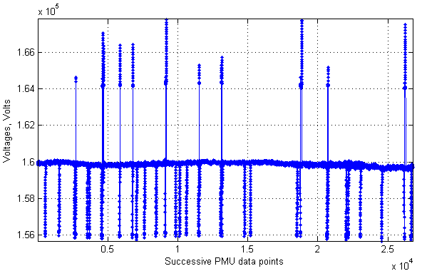
Fig. 1. A signal with many spikes sourced from a PMU
Proposed algorithm for spike detection and removal. The idea is based on computing all signal changes from one measurement to another, and deciding if a specific change was likely to have been caused by a synchronization error or another issue rather than by a power system change of state. In a steady state, voltages and currents usually change in a smooth way so we would not expect to find a sudden «jump». As can be seen in Fig. 1, the data points are concentrated around the value of 1.6 ∙ 105 Volts most of the time. This means that signal point-to-point changes i. e. the gaps between any two adjacent points (which will be referred to as «fluctuations») are expected to take on a rather narrow set of values. In order to decide whether a fluctuation is reliable enough, some criterion should be specified. Based on that criterion, a particular fluctuation can then be compared to what is considered «normal» signal behavior. The author has suggested using either the mean or the median of the absolute values of all calculated fluctuations. Both are common estimators of statistical properties of a large set of data. The mean or the median is then multiplied by a coefficient greater than 1 to set a threshold separating «normal» and suspicious fluctuations.
In order to obtain a good estimate of a typical fluctuation, a relatively large amount of data (at least several thousand points) has to be processed. Otherwise, statistical analysis may not be as correct, which could result in either not detecting spikes well or filtering out too many «good» measurements. It should be noted that even if we deal with a large array of data, there is no guarantee that all outliers will be detected and removed with 100 % accuracy unless all such points clearly stand out against the other data, most importantly, from a mathematical viewpoint. However, the proposed technique allows rejecting most of the outliers in a given signal provided that a proper threshold is chosen. Some comments on how to select a threshold are presented in this paper as well.
A flow chart representing the main steps of signal processing according to the developed algorithm is shown in Fig. 2. We will now discuss some of those steps by referring to the numbered flow chart blocks (see Fig. 2).
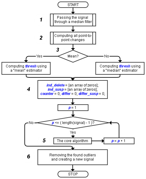
Fig. 2. A flow chart representing the main signal processing steps taken by the developed procedure for spike detection and removal
The first step (block 1 in Fig. 2) is passing the signal through a median filter to remove the very first spike if it happens to be at the beginning of the data set. A proper reference is needed for our core algorithm (block 5 in Fig. 2) from the very beginning so the first point must be a «normal» measurement, not an outlier. Since there is no guarantee the signal starts with a «good» element, the only possible way to set a reference is smoothing out the signal beginning with a median filter. Such filters are particularly effective at and often used for removing impulse noise from experimental data [9, 10]. Note that we cannot just pass a signal through a median filter to achieve our goal of spike detection and removal: along with removing the spiky parts, the filter would also modify all the «good» points. We should therefore do the following:
a) apply a long enough median filter to the whole signal. The filter length should be equal to (2 ∙ N + 1), where «N« is the maximum expected duration of a typical spike;
b) replace the first (N + 1) points in the original signal with those outputted by the median filter; as a result, the first point in the new signal should be safe enough to start looking for spikes from;
c) after the whole signal has been processed, the first (N + 1) points should be cut off, as those points did not belong to the original signal.
As can be seen, we sacrifice the signal beginning to ensure a good performance of the developed spike removal algorithm. Based on some analysis of a large set of real data taken from PMUs, we can conclude that a spike usually lasts for less than 200 successive points, which covers several seconds of measurements with a sampling rate of 30 points per second. At the same time, signals that have been analyzed contain more than 20,000 samples (hereafter the terms «point», «measurement», «sample», and «element» will be used interchangeably). Therefore we do not lose much of the original information anyway.
Block 2 in Fig. 2 represents a call to a subroutine computing all fluctuations i. e. the differences between every two adjacent points. The procedure is straightforward and does not require additional comments.
Conditional block 3 allows the user to select the estimator which will be utilized to analyze all the fluctuations and decide whether a specific fluctuation is «normal» or not. As stated earlier, the threshold «thresh» is either the mean or the median of the absolute values of all the calculated fluctuations multiplied by a coefficient greater than 1. It is suggested that the median be used most of the time, as a median estimator is known for its robustness in the presence of outliers. The median is not as sensitive to outliers in the data compared with the mean value. For us, this means the median will tolerate many spikes in a signal without significantly changing «thresh». However, the developed procedure includes the mean estimator as an option.
Block 4 is where the initialization of some variables relevant to the main algorithm (block 5) takes place. Let us describe the meanings of those variables.
Whenever a big fluctuation is found (greater than «thresh»), it is not necessarily an indicator of an outlier. Although currents and voltages generally change in a smooth way, they could sometimes experience a bigger «jump», or a transition to another level, after which the signal goes smoothly for a long time again. An example of such behavior is shown in Fig. 3. It is therefore necessary to distinguish a real spike from a sudden change of the power system state leading to the signal «jumps». To cope with this issue, the developed procedure analyzes the length of the suspicious signal part. If it is long enough (longer than the length of a typical spiky part), it will not be cut off from the signal.
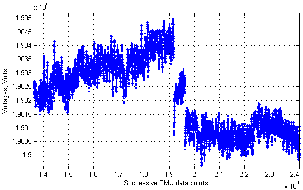
Fig. 3. An example of a «jump» in a voltage signal representing a transition to a new level
One more complication has to be addressed: there could be outliers inside a suspicious group of points. If the group does not get removed from the signal, any spikes found within the group must be filtered out. This brings us to the necessity of keeping track of two types of element indices: «ind_delete» for the elements to be rejected without hesitation, and «ind_susp» for the elements to be removed from a suspicious group of points if the group is not considered as a spike because of its long duration. The «counter» variable counts the number of suspicious points in succession. The other two variables in block 4 (Fig. 2) have the following meanings: «differ» is the difference between a point inside a suspicious group and the last accepted point which does not belong to the suspicious group (a «global» difference), and «differ_susp» is the difference between a point inside a suspicious group and the last point in the same group that will be kept if the whole group is not rejected, which is only possible if its length exceeds that of a typical spike (a «local» difference).
In block 6, all the found spikes get cut off along with the first (N + 1) points, and a spike-free signal (which is always shorter than the original signal) is created.
Let us now outline what happens in the main part of the proposed algorithm (block 5 in Fig. 2). A flow chart showing the sequence of actions hidden by block 5 is presented in Fig. 4.
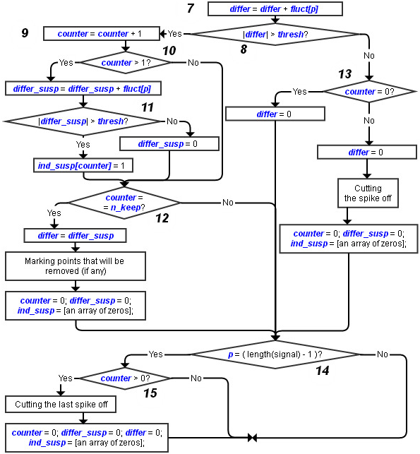
Fig. 4. A flow chart of the core of the proposed technique for spike detection and removal
In block 7 (Fig. 4), the «global» difference is updated so we know the gap between a current point and the last accepted measurement.
Conditional block 8 compares the absolute value of the «global» difference with the threshold. If the former is greater than the latter, a point in a suspicious group is being processed. After updating the counter in block 9, another decision is to be made. If «counter» is greater than 1 (block 10), the suspicious group was detected at an earlier iteration so we can now update the «local» difference and look for outliers within such a group. If the «local» difference «differ_susp» happens to be greater than the threshold (conditional block 11), the end point corresponding to the considered fluctuation «fluct [p]" will definitely be removed from the signal. If the condition is false, the local difference is set back to zero, and the mentioned end point will be a new reference at the next iteration provided that the algorithm goes through the same branches.
Block 12 checks whether the counter has reached «n_keep» — the minimum number of elements following one another, in which case the current suspicious group will not be considered as a spike. The parameter «n_keep» should be set greater than the length of a typical spike. If the condition in block 12 is true, we update the «global» difference, mark the spikes found in the suspicious group, as well as set «counter», «differ_susp», and «ind_susp» back to zeros. Note that «differ» in this case is not assigned a value of zero. Instead, we take into account that several last samples (or the very last one) in the suspicious group might be regarded as outliers, which means they will be removed while the other points in the group kept. The «global» difference in such a situation must inherit the current value of the «local» difference.
The condition in block 13 is checked if the «global» difference «differ» is not greater than the threshold (block 8). This means either that a new suspicious group of points has not yet been found, or that the end of a spike has been detected. If the former is true («counter» equals zero), we simply set the «global» difference to zero so we can get the correct reference before going to the next fluctuation. If «counter» is at least one, the most recently found suspicious group was indeed a spike so the indices of the elements making up the spike will be recorded in order to cut the spike off from the signal. The parameters «differ», «differ_susp», «counter», and «ind_susp» are set back to zeros.
The very last fluctuation has to be analyzed separately (conditional block 14). Otherwise, the last spike will not be filtered out. If «counter» is not equal to zero (block 15), both of the following statements are true: 1) the algorithm has been processing a suspicious group of points; 2) «counter» has not reached «n_keep». The last suspicious group is therefore considered as a spike and should be removed from the signal.
Simulations and results. This section presents some case studies showing the effectiveness of the proposed technique for spike detection and removal. The algorithm of Fig. 2 and 4 has been implemented in MATLAB as a set of m-files.
In order to verify the algorithm before applying it to measurements outputted by PMUs, the author came up with a test signal containing both spikes (should be cut off) and abrupt transitions (should be retained). The signal consists of 200 samples, most of which are pseudorandom numbers generated from the uniform distribution on the interval [-0.5, 0.5]. All the signal elements from 1 to 200 are presented in Table 1. The generated random numbers are called «rand» without specifying the exact values.
Table 1
The elements of a basic test signal created in order to verify the proposed algorithm
|
1 |
2 |
3 |
4 |
5 |
6 |
7 |
8 |
9 |
10 |
11 |
12 |
13 |
14 |
15 |
16 |
17 |
18 |
19 |
20 |
|
rand + 1 |
3.5 |
3.8 |
4.1 |
rand + 4 |
3.3 |
1.3 |
rand + 1 |
||||||||||||
|
21 |
22 |
23 |
24 |
25 |
26 |
27 |
28 |
29 |
30 |
31 |
32 |
33 |
34 |
35 |
36 |
37 |
38 |
39 |
40 |
|
rand + 1 |
|||||||||||||||||||
|
41 |
42 |
43 |
44 |
45 |
46 |
47 |
48 |
49 |
50 |
51 |
52 |
53 |
54 |
55 |
56 |
57 |
58 |
59 |
60 |
|
rand + 1 |
|||||||||||||||||||
|
61 |
62 |
63 |
64 |
65 |
66 |
67 |
68 |
69 |
70 |
71 |
72 |
73 |
74 |
75 |
76 |
77 |
78 |
79 |
80 |
|
rand + 1 |
-9 |
-8.5 |
-8 |
-2 |
0.5 |
-0.1 |
rand — 4 |
-12 |
rand — 4 |
-6.5 |
-7.3 |
rand — 4 |
|||||||
|
81 |
82 |
83 |
84 |
85 |
86 |
87 |
88 |
89 |
90 |
91 |
92 |
93 |
94 |
95 |
96 |
97 |
98 |
99 |
100 |
|
rand — 4 |
|||||||||||||||||||
|
101 |
102 |
103 |
104 |
105 |
106 |
107 |
108 |
109 |
110 |
111 |
112 |
113 |
114 |
115 |
116 |
117 |
118 |
119 |
120 |
|
-3 |
-3.1 |
-3.2 |
-3.3 |
rand — 4 |
|||||||||||||||
|
121 |
122 |
123 |
124 |
125 |
126 |
127 |
128 |
129 |
130 |
131 |
132 |
133 |
134 |
135 |
136 |
137 |
138 |
139 |
140 |
|
rand — 4 |
|||||||||||||||||||
|
141 |
142 |
143 |
144 |
145 |
146 |
147 |
148 |
149 |
150 |
151 |
152 |
153 |
154 |
155 |
156 |
157 |
158 |
159 |
160 |
|
rand — 4 |
-6 |
-5.9 |
rand — 4 |
||||||||||||||||
|
161 |
162 |
163 |
164 |
165 |
166 |
167 |
168 |
169 |
170 |
171 |
172 |
173 |
174 |
175 |
176 |
177 |
178 |
179 |
180 |
|
rand — 4 |
rand |
4 |
rand |
||||||||||||||||
|
181 |
182 |
183 |
184 |
185 |
186 |
187 |
188 |
189 |
190 |
191 |
192 |
193 |
194 |
195 |
196 |
197 |
198 |
199 |
200 |
|
3.5 |
4.5 |
rand |
-5 |
rand |
|||||||||||||||
Assuming that a spike cannot last longer than 10 samples, we set «n_keep» (see block 12 in Fig. 4) equal to 10. The most important decision is selecting an estimator and a threshold that will allow the algorithm to remove the spiky parts effectively while keeping most (if not all) of the «good» points. As previously mentioned, the median estimator is generally preferable to the mean one. A proper threshold should usually be several times greater than the median of the absolute values of all computed fluctuations. For our basic test signal with the elements shown in Table 1, a threshold equal to five times the median works well. For a real signal sourced from a PMU and containing thousands of samples, the use of statistics becomes more effective, which makes it easier to choose a good enough threshold. Let us discuss this in more detail later.
Fig. 5 shows the result of applying the developed algorithm to the test signal. As can be seen from the figure, the algorithm has successfully detected all the outliers which were deliberately put into the signal. The bold lines indicate the new connections after removing the spikes. Certainly, the improved signal will contain fewer points than the original one. Note that the first 11 points are discarded anyway, which is clearly shown in Fig. 5. The reason for such a result, as explained earlier, is that the first (N + 1) points (with «N« equal to 10 in this case) are replaced by those outputted by a median filter (see block 1 in Fig. 2).
A more interesting example is presented in Fig. 6. Here, we insert 20 more points in our basic test signal (Table 1). A set of values {7.1, 7, 4.2, 2.3, 2, 1.7} goes to the beginning of the signal while a set {4, 4.2, 4.4, 4.6, 4.8, -3, 5, 5.2, 5.4, -4, -3.75, -3.5, -3.25, -3} is appended to the end of it. As shown in Fig. 6, all the outliers, including those at the left and right borders, have been found.
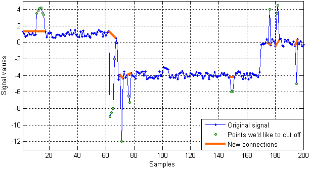
Fig. 5. An illustration of the algorithm performance for the test signal of Table 1
The developed technique has also been tested on a variety of real current and voltage signals acquired from PMUs. As an example, let us consider the imaginary part of a current signal measured in phase A on a 345 kV transmission line. The original signal supplied to our algorithm is comprised of 26,772 samples. Based on some analysis of a large amount of different signals measured on the same line, we came to the conclusion that a spike cannot last for more than 200 samples so «n_keep» (see block 12 in Fig. 4) was set equal to 200.
Since the signal is relatively long, some useful statistics can be derived. It turns out that point-to-point differences (fluctuations) in this and many other signals measured by PMUs have a distribution close to normal (Gaussian) if the biggest fluctuations are not taken into consideration. The standard deviation of normally distributed data can be estimated using the median absolute deviation (MAD) multiplied by a constant scale factor equal to 1.4826 [11]. This estimator is known to be resilient to outliers in the data, which is typical of median-based estimators. Let us estimate the standard deviation of all fluctuations for our signal through the MAD, and then discard all of the fluctuations that are three or more standard deviations away from the mean. The remaining fluctuations (96.3 % of the total amount) will have a nearly normal distribution (Fig. 7). That is confirmed by the kurtosis and skewness values equal to 3.23 and 0.08, respectively.
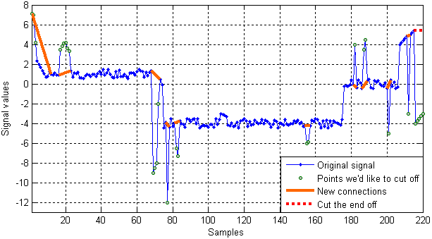
Fig. 6. An illustration of the algorithm performance for an extended test signal with spikes at the beginning and end
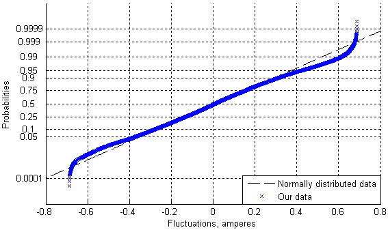
Fig. 7. The statistical distribution of most of the fluctuations for a real signal
This last example shows that fluctuations derived from steady state PMU measurements can be assumed to have a distribution close to Gaussian. Such a conclusion makes it easy enough to choose a threshold for our spike removal algorithm. A threshold of (5 × 1.4826 × the MAD) appears to be safe enough since a particular point drawn from a normal distribution is rarely more than a few standard deviations away from the mean. Using such a threshold for our signal made up of 26,772 samples, we can say that the spiky parts have been detected effectively (Fig. 8), and the improved signal obtained after removing 2,994 points looks much smoother than the original one (Fig. 9).
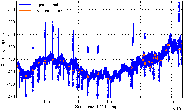
Fig. 8. An illustration of the algorithm performance for a real signal (the detected spikes are highlighted)
Conclusion. This paper presents an algorithm for the automatic removal of spikes from steady state current and voltage measurements coming from phasor measurement units. It has been shown that the developed algorithm performs well when processing both simulated and real signals. It is generally hard to discard spikes with 100 % accuracy unless all the spiky parts clearly stand out against the other points. However, some recommendations on how to select a proper threshold when dealing with a large set of real data are provided in the paper. These recommendations are confirmed by the results presented in Fig. 8 and 9.
Acknowledgement. The author would like to thank the American Transmission Company (the USA) for providing a large array of PMU data used for analysis.
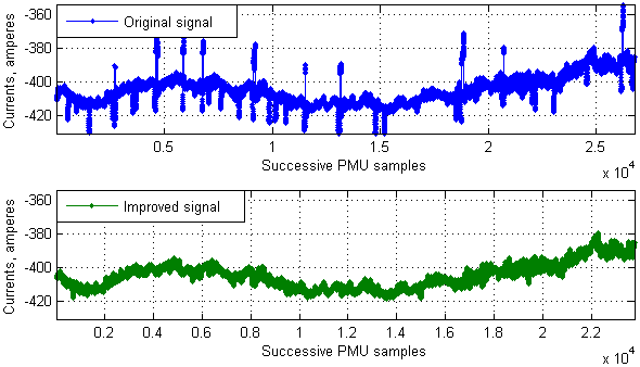
Fig. 9. A real signal with spikes (the top plot) and the same signal after being processed by the developed algorithm (the bottom plot)
References:
1. D. G. Hart, D. Uy, V. Gharpure, D. Novosel, D. Karlsson, and M. Kaba, «PMUs — A new approach to power network monitoring», ABB Review 1/2001. Available at: http://www05.abb.com/global/scot/scot296.nsf/veritydisplay/2d4253f3c1bff3c0c12572430075caa7/ (Accessed: 31 July 2014).
2. B. Singh, N. K. Sharma, A. N. Tiwari, K. S. Verma, and S. N. Singh, «Applications of phasor measurement units (PMUs) in electric power system networks incorporated with FACTS controllers», International Journal of Engineering, Science and Technology, vol. 3, no. 3, pp. 64–82, 2011.
3. M. Adamiak, W. Premerlani, and B. Kasztenny, «Synchrophasors: definition, measurement, and application», Protection and Control Journal, GE Multilin, pp. 57–62, September 2006.
4. А. G. Phadke and J. S. Thorp, Synchronized Phasor Measurements and Their Applications. Springer, 2008.
5. S. Chakrabarti, E. Kyriakides, T. Bi, D. Cai, and V. Terzija, «Measurements get together», IEEE Power and Energy Magazine, Jan.-Feb. 2009. Reprinted in Special Issue: Smart Grid-Putting it All Together, a 2010 reprint journal from PES, pp. 15–23.
6. T. Bi, H. Liu, X. Zhou, and Q. Yang, «Impact of transient response of instrument transformers on phasor measurements», in Proc. 2010 IEEE PES General Meeting, Minneapolis, MN, USA, July 25–29, 2010.
7. Schweitzer Engineering Laboratories, Inc. (2008), «SEL synchrophasors — A new view of the power system». Available at: https://www.selinc.com/WorkArea/DownloadAsset.aspx?id=132 (Accessed: 31 July 2014).
8. Y. Liao and M. Kezunovic, «Online optimal transmission line parameter estimation for relaying applications», IEEE Transactions on Power Delivery, vol. 24, no. 1, pp. 96–102, January 2009.
9. D. C. Stone, «Application of median filtering to noisy data», Canadian Journal of Chemistry, vol. 73, no. 10, pp. 1573–1581, 1995.
10. J. Micek, J. Kapitulik, «Median filter», Journal of Information, Control and Management Systems, vol. 1, no. 2, pp. 51–56, 2003.
11. J. S. Walker, A Primer on Wavelets and Their Scientific Applications. Chapman & Hall/CRC, Taylor & Francis Group; 2 edition, 2008.
