Prediction of CO2 emission based on the NARX neural network of Iraq



Environmental improvement steps are important factors in relation to technological progress in the world, and it is considered one of the fierce enemies of the environment, one of its tools is carbon dioxide (CO ₂ ) emissions as it is an indicator of environmental pollution with its high rates in the atmosphere, and predicting its emissions and future expectations contribute greatly to drawing up a sustainable environmental policy. On this basis, this study used one of the most important artificial intelligence (AI) tools, which is the multilayer nonlinear autoregressive exogenous model (ML-NARX), to predict and forecast annual CO ₂ emissions and their quantities in Iraq until 2032. The measured CO ₂ emissions data were collected for the purpose of studying from the «Our World in Data» website from 1950 to 2022 because some previous measurements were missing, as the database consisted of 73 samples that were divided into a training set, a test set, and a validation set at a ratio of 70:15:15, respectively. The proposed model was designed to consist of two hidden layers and the effect of modifying the number of nodes in each of the two hidden layers on the accuracy of the prediction was studied. As for the inputs used, one set was formed to predict the next value from the past value based on the time sequence of CO ₂ emission years. Mean Squared Error (MSE) and Root Mean Squared Error (RMSE) were adopted as performance measures in evaluating the model, as the network was trained to reach the lowest value of MSE and RMSE which were 6.46E-04 and 2.54E-02 respectively, and the best structure used for the model was determined to be (10) nodes in first layer and (25) nodes in second layer. The output of the model's prediction curve for ten years for CO ₂ emission for the period from 2023 to 2032 showed an increase at a rate of 1.7820 million tons/year. Therefore, the results of this work will help local government and decision-makers to take the necessary and wise measures to address the environmental reality for the near and distant future as well.

Keywords: prediction, ML-NARX, CO ₂ emission, time series.

1. Introduction

The alarming level of CO ₂ emissions into the atmosphere is a concerning indication, since the rapid rise of the global population has greatly contributed to an increase in carbon emissions owing to human wants and needs [1]. High levels of CO ₂ have had a significant and direct impact on Earth's climate. This includes the increase in global temperatures due to global warming in the atmosphere, the expansion of land without trees due to population growth, changes in rainfall patterns and agricultural productivity, increased ocean acidity, and water scarcity. These factors have a direct impact on human health, leading to higher rates of various diseases [2, 3]. Following the 1960s, there was an increase in CO ₂ emissions worldwide, coinciding with economic expansion in all nations. This economic growth led to a significant increase in industry and its diversification. Iraq is a significant oil-producing nation globally [4, 5], consequently, the extraction and refining processes necessary for manufacturing different petroleum derivatives result in the emission of substantial amounts of CO ₂ .

The State of Iraq, situated in a geographically unique region, experiences extremely high temperatures. Recent measurements have shown an average temperature increase to 50 degrees Celsius on certain days [6]. Additionally, the region has a dry atmosphere and is prone to dust storms during the summer. The occurrence of climate changes worldwide is attributed to the escalating release of CO ₂ and methane, along with other gases existing in the atmosphere. These gases, known as greenhouse gases or global warming agents, contribute to the rise in the Earth's surface temperature [7]. These causes have significantly contributed to climate change in Iraq, aligning with global climate change. This will result in economic loss as the yearly levels of greenhouse gases continue to increase [8].

Reports reveal a high prevalence of severe illnesses and chronic health conditions resulting from air pollution, ultimately leading to fatalities. The World Health Organization's yearly global figures indicate that almost 7 million individuals have died [9]. The large increase in the amount of CO ₂ and other pollutants is mostly linked to the large increase in industrial activities, cars and energy production, in addition to deforestation, which coincides with the population expansion resulting from the increase in human density in the world. [10]. Therefore, it is important to prioritize finding effective solutions to reduce local CO ₂ emissions in order to address this issue before decision — makers.

Utilizing AI techniques to predict CO ₂ gas emissions is an effective approach for assessing the future consequences of emissions [11]. This method provides a comprehensive understanding of the magnitude of the issue and its overall environmental implications. Additionally, it enhances public awareness and facilitates the development of proactive strategies to mitigate future risks.

AI has proven to be highly effective in analyzing, detecting, and predicting data [12], utilizing machine learning algorithms, deep learning, and transfer learning. It has made significant contributions across various fields [13] and has also played a role in establishing strategies for reducing CO ₂ emissions. Including AI predicting and forecasting model for time series NARX, due to the need for precise calibration and adherence to high criteria regarding the training and testing data, the employment of this method might yield promising outcomes.

Future projections can be used to understand the issue of emissions and assess its impact, these projections will enable us to see the developments that will appear in the long term and allow Iraqi government agencies to implement supportive policies. These policies can effectively prevent the escalation of emissions rates or explore alternative ways to reduce them, Especially since the gradual rise in temperature in Iraq, together with the significant releases resulting from oil refining, burning oil derivatives, and emissions from industrial areas, these factors will provide a genuine risk to the health, ecology, and economy [14].

This work provides an overview of the model utilized in this study and the resulting outcomes. It also explores the potential for revising the forecasts generated by this model to incorporate additional data, such as technological advancements, industrial growth, population growth, and the future implications of new technologies. By doing so, it aims to assess the effectiveness of the policies implemented in terms of their impact on CO ₂ levels, whether positive or negative. This work conducted a multi-level analysis of the model used to predict CO ₂ emissions. The study focused on evaluating the accuracy of this model and aims to serve as a valuable resource for future researchers who wish to compare them with other comparable forecasting models.

The remaining sections of the paper are structured in the following manner: The literature review section focuses on scholarly publications about the topic of CO ₂ emissions and forecasting, as well as related studies. The section on the data set provides information regarding its origin and a detailed analysis of its characteristics. The section on the suggested methodology provides a description of the proposed model and the performance indicators utilized for evaluation. The Performance Analysis section is a comparative assessment of current efforts, focusing on an analysis of the model's performance. In the part dedicated to the conclusion and future study directions, the author presents the political implications, future research directions, and the limits associated with them.

A comprehensive study was conducted to examine various concerns pertaining to CO ₂ emissions and their long-term consequences. As a result, alternative solutions were identified, and there has been a growing inclination towards using advanced technology to develop future strategies and goals. Recent research on time series data of CO ₂ emission have showcased the application of AI, including statistical models, machine learning, and deep learning, to determine the most effective method for predicting and assessing future trends. Hence, it is feasible to discern a cluster of research endeavours that focus on this domain and its diverse prognostication techniques.

In their study, R. P. Masini et al. [15] focused on the use of machine learning and high-dimensional supervised models for predicting supervised time series. They employed both non-linear and linear approaches, combining hybrid and ensemble models from several options. Furthermore, time series projections have been implemented in the realm of finance and economics.

R. Mustakim et al. [16] worked on using two non-linear neural networks, namely Support Vector Regression (SVR) and NARX Neural Network to predict the air quality index and the effects of pollution on the economy and public health. also used four aspects of implementation: parameter selection, robustness, input re-preprocessing, and practical predictability limit. The results of the comparison between the two models showed convergence in the prediction process, but the SVR model outperformed the other model NARX.

A. H. Bukhari et al. [17] designed a hybrid computing model using the fractional order Lorenz-based physics information and NARX and seasonal autoregressive fractionally integrated moving average (SARFIMA) model to predict the hourly pattern from the previous two days. It uses weather forecasts and the Earth's dynamic system in combination with physical, biological, and chemical processes within the laws of various sciences, in addition to the information available through physical intelligence about climate variation. The proposed model showed efficiency for early pattern prediction at the expense of statistical indicators based on computational intelligence in monitoring the environment and air pollution. H. Jung and J. H. Lee [18] used a design that uses NARX with Model predictive control (MPC) as a general prediction model (NARX-MPC), in a move to control the dynamic operating environment contributed by Post-combustion CO ₂ capture (PCC). The proposed model is evaluated with another model represented by linear MPC (LMPC), where NARX-MPC outperforms the other model in performance in closed-loop control in terms of changes in the flow rate of CO ₂ and flue gas, as well as changes in the load of the power plant.

D. Ma et al. [19] proposed working on a time series model to identify and predict changes in CO ₂ levels in the atmosphere. The NARX model was applied in the forecasting process, where it conducted experiments on manually releasing CO ₂ and monitored the behaviour of the proposed model with the leakage signal occurring. The proposed model showed excellent prediction for capturing the signal of CO ₂ leakage into the atmosphere in abnormal cases.

M. Mutascu [20] Their work aims to predict CO ₂ emissions within fourteen categories of renewable energy consumption, based on a combination of vector autoregressive (VAR) and artificial neural network (ANN) models. The estimates were based on ten different types of inputs to the model for the period from 1984 to 2020, and the accuracy of the ANN model was higher compared to the other model, but the superiority of this network faced difficulties in sudden and sharp indicators in the accuracy of production. In addition, the accuracy of predicting the emission of dioxide increased during the period of epidemiological crises as an effective element in contributing to decision-making.

M. Ahad [21] They used a new approach to detect CO ₂ emission levels in Pakistan, represented by quantile regression, which performs a quantitative causal analysis of non-renewable energy sources and the correlation of their effect to long-term levels compared to renewable energy sources. Analytical results for the period from 1972 to 2020 revealed that renewable energy sources positively affect CO ₂ emission, They used a new approach to detect CO ₂ emission levels in Pakistan, represented by quantile regression, which performs a quantitative causal analysis of non-renewable energy sources and the correlation of their effect to long-term levels compared to renewable energy sources. Analytical results for the period from 1972 to 2020 revealed that renewable energy sources positively affect the emission of CO ₂ , as it demonstrated a bidirectional causal relationship for energy consumption, high emissions, and consumption of non-renewable and renewable energy through their highest and lowest quantities.

J. M. S. Sama et al. [22] predicted the symmetric and asymmetric impact on crude oil production (COP) by using recorded indices from 1977 to 2019 of CO ₂ emission, economic, inflation, and human development index (HDI) in Cameroon. They used the non-linear autoregressive distributed lag (NARDL) and autoregressive distributed lag (ARDL) models to evaluate the symmetrical and asymmetric effects. The results showed that CO ₂ emission and economic growth in the long term had a negative impact on COP, while inflation and HDI indicators had a positive impact in the short term. There was an asymmetric effect of the economic growth indicators and HDI in the short term, and in the long term, there was an asymmetric effect on the COP through the inflation and CO ₂ emission indicators.

The objective of this study is to look at CO ₂ emissions in Iraq from 1953 to 2020 and provide predictions for the future using machine learning methods. Two models were created to forecast CO ₂ emissions using time series data, and the most accurate model was selected based on the precision of its predictions. Furthermore, these forthcoming forecasts of CO ₂ emissions offer a valuable understanding of the severity of this issue and its future impact on the region's climate. They also aid in promoting strategies to address environmental and economic challenges by formulating effective plans and policies to mitigate the excessive emission rates in the area.

2. Material and methods
   1. Dataset

This study utilized a comprehensive dataset of CO ₂ emissions for Iraq over 73 years, specifically from 1950 to 2022. The dataset was obtained from a reliable repository (Our World in Data) [23–25], and its accuracy was confirmed by verifying the models used. This analysis employs the univariate time series data of Iraq, which demonstrates a persistently rising trajectory in CO ₂ emissions, Figure 1 depicts the emission of CO ₂ intensity in Iraq from 1950 to 2022.

Data pre-processing is performed before splitting the data into training and testing sets. Assessing the performance of a model entails utilizing test data to evaluate the accuracy and efficacy of the model. Subsequently, models with exceptional performance are employed to forecast CO ₂ emissions. The data has undergone processing, engineering, and organization.

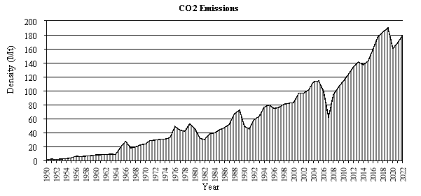
Fig. 1. Plot of CO ₂ emissions of Iraq, measured in millions of metric tonnes per capita, from 1950 to 2022.

Due to the presence of impurities such as missing values (NA), special characters, or inaccurate values, it is not feasible to directly utilize the raw data for model training. Consequently, the gathered data is subjected to pre-processing to remove any illogical values and exclude them. Hence, data from the year 1950 onwards was utilized, excluding older years due to data gaps and nonsensical values. This was done to prevent any interference with the training and testing of the model and to maintain the integrity of the model's outputs. The dataset presents CO ₂ emission data, which is displayed in Table 1, and includes a descriptive analysis. After analyzing the minimum, median, and maximum values, it is clear that there is a noticeable rising trend in CO ₂ emissions.

Table 1

Analysis providing data

Variables	Estimate
Count	73
Maximum	189606500
Minimum	1648533
Median	48735490
Mean	64146639.86
Standard error	6182211.53
Standard deviation	52820838.47
Skewness	0.793
Kurtosis	-0.334

The average emissions of CO ₂ reached 64,146,639.86 metric tons per capita, with a maximum emission of CO ₂ reaching 189,606,500 metric tons per capita, and a minimum amounting to 1,648,533 metric tons per capita.

2.2. Input normalized

The data obtained have values of varying scales, and may affect the prediction process in terms of performance [26]. For the purpose of dealing with this data, it is suggested to apply normalization to it [27], where the structure of machine learning is affected by the normalization approach in addition to the specific application [28]. Normalizing inputs leads to added computational burdens, as their estimates must be taken into account correctly [29], but there is a difficulty in real applications. Moreover, it is necessary to convert the resulting values of the forecasting process to the original standards when preparing the report.

Normalization is used using the min-max technique on the input data [30], as Equation 1 is used to calculate its value.

…….(1)

x indicates the original value, indicates the maximum value, and indicates the minimum value of the data.

2.3. Multilayer of NARX (ML-NARX) model

The basic principle of the NARX network is a nonlinear autoregressive exogenous (ARX) model, which is widely used in specifying linear black box systems. It is worth noting that NARX models are widely used to improve and enhance nonlinear descriptive modeling of dynamic systems [31], solar radiation and its prediction mechanism [32], prediction of chaotic time series [33], detection and identification of faults by series-parallel time series [34], long-term and short-term prediction of time series [35]. The dynamic of the recurrent neural network, or what is called NARX, is considered a type of neural network that takes from previous experiences as a method of learning, and the feedback that the network adopts as a basis is characterized by links with multiple levels. The NARX network has two different architectures, called parallel architecture (close loop) and serial parallel architecture (open loop), which are shown in Fig. 2.

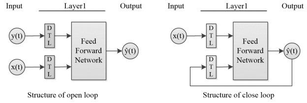
Fig. 2 Architectures of the close and open loops of the NARX neural network

A description of the dynamics of the NARX network is shown as follows by the equation (2) [36]:

……..(2)

Here, the input delay is represented by x(t-n) to the network and the output delay is represented by y(t-n) , and t is referred to as the time period, while 𝑦̂(𝑡+1) is the output of the NARX network at t . with respect to which the function F is the mapping of the neural network. The internal structure of the NARX network consists of several layers, the first of which is the direct input layer of data passing through a time delay vector, secondly the output feedback is also passed through a delay vector where sigmoid activation functions are used, in addition to the weights, which is its other component, and finally the output layer.

Its function lies in the speed of convergence, as the activation functions, including Hyperbolic and Logsigmoid, play an ideal role in the scaling factors, which gives it strength in performance, and as follows the equations (3) and (4) translate the mathematical form of these two functions [37].

….(3)

… (4)

To obtain the most efficient training process for the network, a feedback loop is opened in it, as the real outputs are provided within the stages of the training process. An open loop structure was used, because the estimated outputs are not sent again, but rather the real outputs are used, which in turn provides the network with more accurate inputs.

In this study, it was proposed to work on parallel engineering with the addition of several hidden layers to the NARX model to study the emission of CO ₂ and predict it for several years. The proposed design shows the network structure as in the Fig. 3.

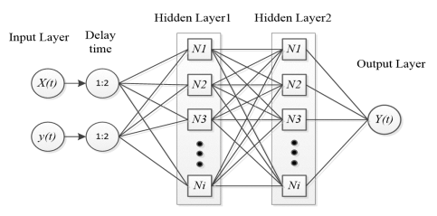
Fig. 3. Proposed model of ML-NARX network

In the experiment, the number of neurons ranged from 5 to 25 in the first and second layers, respectively, with transmission intervals of 5. The purpose was to reach the best performance obtained from the network. The number of delays was set to 2 because it gives results with high accuracy [38]. The data is divided into three groups, which are 70 % training set, 15 % for testing, and 15 % for validation for the prediction process [35]. Table 2 shows the initial parameters used in the proposed model.

Table 2

The initial parameters of ML-NARX

Parameters	Value
Number of neurons in Layer1	5, 10, 15, 20, 25
Number of neurons in Layer2	5, 10, 15, 20, 25
Maximum number of iterations	100
Number of epochs	1000
Delays	1:2
Activation function	sigmoid
Divided dataset to training, testing, and validation	75:15:15

2.4. Predicting for a time series based on future values

Applications are accessed to describe different operations on the NARX network. In the nntrain window, specifically at the top of it, there is a model of a nonlinear autoregressive neural network with external inputs. On the basis of the studied data and its previous values, in addition to the external input signal, the network was modified to include two hidden layers in which the various neurons are alternately applied, and one neuron for the output layer for the prediction process.

were applied A non-linear optimization method was used to train the neural network, with the use of the Levenberg-Macwardt algorithm, which would reach the lowest MSE, as it is a tool to evaluate the performance of the neural network and its results. After dividing the input data into vectors, they are used in the training process for the model and testing for the independent network, verifying reliability and avoiding excessive results for the training process.

In order to predict the vector series for ŷ(t) and obtain the appropriate accuracy for it, as indicated in Equation (2), the prior values ​​x(t) are taken for the real data with an input delay period of n, and an additional measurement series for the input y(t), On the basis of these notations, the time series is designed for predicting.

2.5. Performance measures

The performance of the prediction model is evaluated based on measures to estimate the condition and analyze it as a criterion for performance every time the moment 𝑛 is taken. Among these measures to show the performance are the MSE, the RMSE, regression (R ² ), and the mean absolute error (MAE), and the error histograms, as its mathematical formula is given by the following equations(5–8) [39]:

………………………… (5)

………………………… (6)

………………………….. (7)

…………………………. (8)

Actual values are denoted by , predicted values are denoted by , the number of data points is denoted by j, and is denoted by the expected mean of

values. Based on the performance measures, the best structure for the ML-NARX network is nominated through the best results obtained for predicting CO ₂ emissions, in addition to predicting the next ten years for the nominated structure. The flowchart in Figure (4) shows how the ML-NARX algorithm works.

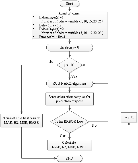
Fig. 4 Flow chart of ML-NARX Algorithm

3. Results and discussion

In this section, the model's neural network is trained through a backpropagation algorithm, to obtain state estimates for the MSE, RMSE, R2, MAE, and error histograms of the proposed ML-NARX network. The work was done in MATLAB to design the structure of the ML-NARX model in the neural network toolbox. The design consisted of one input to the network, two hidden layers, and one output layer, in addition to a feedback path with a delay time of 1:2. The input value of the data is one string for the real state of the passive target for the first layer of the ML-NARX model, and then to the second layer to obtain the prediction outputs for the output layer. In the two hidden layers, the sigmoid function acts as an activation function for the neurons, and the first and second layers consist of a number of nodes to form, starting from (5, 10, 15, 20, and 25) and in simultaneous and consecutive ways to reach the best result for estimating the condition.

Table 3 shows the results of training and testing of the model for the input series with the number of cases in which the number of nodes per layer is permuted.

Table 3

Performance result of ML-NARX

Number of Nodes		Training			Testing
Layer1	Layer2	MSE	MAE	RMSE	MSE	MAE	RMSE
5	5	1.63E-04	6.83E-03	1.28E-02	8.95E-04	2.06E-02	2.99E-02
5	10	6.33E-05	4.62E-03	7.95E-03	6.55E-04	1.54E-02	2.56E-02
5	15	3.96E-06	7.68E-04	1.99E-03	9.20E-04	2.04E-02	3.03E-02
5	20	2.12E-06	4.61E-04	1.45E-03	9.01E-04	1.75E-02	3.00E-02
5	25	4.03E-16	1.51E-08	2.01E-08	8.64E-04	1.95E-02	2.94E-02
10	5	4.80E-05	2.93E-03	6.93E-03	8.84E-04	1.93E-02	2.97E-02
10	10	2.12E-06	4.34E-04	1.45E-03	1.00E-03	2.04E-02	3.16E-02
10	15	1.13E-08	3.30E-05	1.06E-04	8.58E-04	2.36E-02	2.93E-02
10	20	9.88E-17	7.20E-09	9.94E-09	9.59E-04	1.97E-02	3.10E-02
10	25	3.65E-24	1.42E-12	1.91E-12	6.46E-04	1.55E-02	2.54E-02
15	5	1.30E-06	3.71E-04	1.14E-03	9.49E-04	1.72E-02	3.08E-02
15	10	1.51E-07	1.95E-04	3.89E-04	9.34E-04	1.94E-02	3.06E-02
15	15	3.14E-10	4.61E-06	1.77E-05	8.69E-04	1.84E-02	2.95E-02
15	20	1.90E-07	1.37E-04	4.35E-04	9.92E-04	2.17E-02	3.15E-02
15	25	3.02E-07	1.80E-04	5.49E-04	9.00E-04	1.79E-02	3.00E-02
20	5	1.28E-07	1.20E-04	3.58E-04	8.13E-04	2.11E-02	2.85E-02
20	10	1.12E-08	3.73E-05	1.06E-04	8.82E-04	1.88E-02	2.97E-02
20	15	1.31E-08	3.79E-05	1.14E-04	8.08E-04	2.14E-02	2.84E-02
20	20	3.26E-19	4.39E-10	5.71E-10	8.75E-04	2.06E-02	2.96E-02
20	25	2.21E-18	1.11E-09	1.49E-09	7.47E-04	2.17E-02	2.73E-02
25	5	3.19E-06	5.46E-04	1.79E-03	7.07E-04	1.90E-02	2.66E-02
25	10	2.84E-08	5.23E-05	1.69E-04	8.62E-04	2.41E-02	2.94E-02
25	15	4.66E-08	7.37E-05	2.16E-04	8.10E-04	1.77E-02	2.85E-02
25	20	4.41E-08	6.09E-05	2.10E-04	6.93E-04	1.67E-02	2.63E-02
25	25	1.19E-23	1.89E-12	3.45E-12	7.29E-04	1.83E-02	2.70E-02

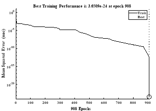
Through the results obtained in table 3 and comparing the results with each other, it found that the best design for the model is at (10) nodes in first layer and (25) nodes in second layer, based on the lowest value obtained for the MSE, which is 6.46E-04, as well as the RMSE is 2.54E-02 in the testing process, additional, the training process of the proposed model, all data were trained, the results of its performance metrics were shown. obtained lowest value in the training process to MSE, MAE, and RMSE is (3.65E-24, 1.42E-12, and 1.91E-12) respectively.

Compared to the two layers (5 10) in the testing process, which obtained the lowest MAE value and amounted to 1.54E-02, and for the MSE and RMSE, their values reached respectively 6.55E-04 and 2.56E-02, which is higher than the value of the two layers (10 25), and, as for the training process, the results for the performance measures were higher than the two layers (10 25).

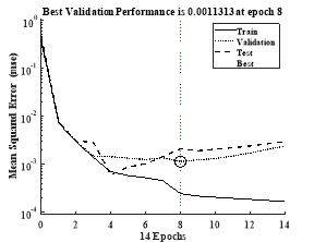
In light of these results, Choose the design of the structural model (10 25) to list the results related to it, Fig. 5.a show the training phase and Fig. 5.b show the testing phase of the model in light of the three divisions, which are the training data set 70 %, the test 15 %, and the validation 15 %, in addition to training the network on 1000 epochs to reach the best performance, as shown by the convergence curves among a set of permutations of the number of nodes in the two hidden layers.

(a) training process (b) testing process

Fig. 5. The performance of ML-NARX model, (a) training, (b) testing

Fig. 6 shows the ML-NARX model, which includes the results of the regression, which represents a combination of statistical operations between the target variable y(t) and the output variables ŷ and the correspondence between them to reach the prediction. In light of dividing the data set into 75 % for training, 15 % for testing, and 15 % for verification, the R2 reference is 0.991 and 0.997 for training the model, 0.968 for testing, and 0.989 for verification, which indicates good performance due to the lack of overfitting through the convergent linear behavior between the output and target values.

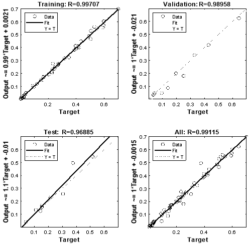
Fig. 6. The Correlation coefficient of ML-NARX model

Fig. 7 shows the histogram of errors between the target values ​​y(t), y(t-1) and the estimated target value ŷ for the ML-NARX algorithm after the training, testing and validation process, where the local system error estimates were close to zero and these errors can be negative. The total error is represented by twenty vertical bars of the neural network called candles, and each candle indicates a number of points extracted from the total data set on the y-axis. These bars are centered by candles that correspond to the error, and the closer the bars on the x-axis are to the center, the smaller the error percentage, while the height of the candle indicates the total training, testing and validation data that are within a certain range of errors and are called frequencies.

The number of error repetitions was 19 times for the training process, 22 times for the validation process and 24 times for the testing process between -0.00113 and 0. Then the number of error frequencies between 0 and -0.01064 decreased to 3 times for the training process, 4 times for the validation process, and 6 times for the testing process, until it reached a frequency of one error between 0 and -1152. As for the number of error frequencies between 0 and 0.00837, it reached 9 times for the training process and 10 times for the validation process, until the number of error frequencies reached a frequency of one for the validation process between 0 and 0.06541.

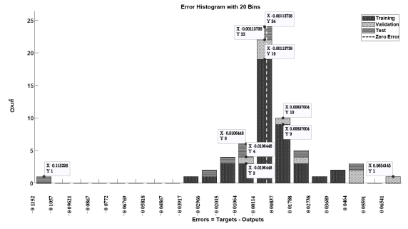
Fig. 7. The error histogram for training, validation, and testing of ML-NARX model

Fig. 8 shows the errors of the training, testing and validation process for the ML-NARX algorithm and the real data of the input data set, where the highest error value (-0.1199) was at sample 37, followed by sample 24, which had a value of 0.0701, while the rest of the errors ranged between (0.0504) and (-0.0437).

Fig. 8. The error for Training, validation, and Testing of ML-NARX model

Fig. 9 depicts the autocorrelation of the ML-NARX model performance, which helps to give a picture of the nature of the data and the mechanism of modeling it in time series, in addition to how the sequence of observations of the data affects the enhancement of the generalization of the model through the dependence of the data among them, and that the power of predicting CO ₂ emissions is originally due to the improved generalization of the model. For the purpose of analyzing the time series with their lagged values, autocorrelation is mostly used. It gives a good indicator if the autocorrelations are within the 95 % confidence interval, which is an indication of the occurrence of the white noise process for the model, although the lag stages in addition to the automatic errors are below the 95 % confidence interval.

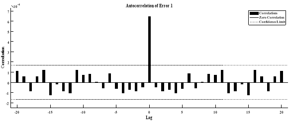
Fig. 9. The autocorrelation of error for ML-NARX model

Using the ML-NARX model for the training and response process and the required initial weights setting mechanism by trial and error, the time series plot of the test data is shown in Fig. 10, showing some time steps that have major errors but are generally acceptable, as it shows the predictions for CO ₂ , which is what was obtained for the lowest MSE of the permutation process with the number of nodes for the hidden layers, which is 6.46E-04.

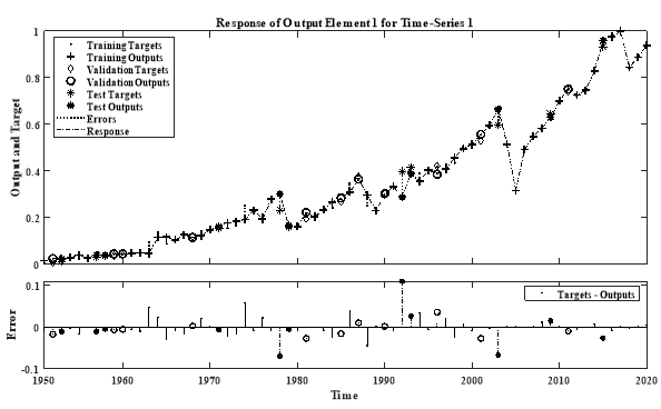
Fig. 10. The time-series of predicted and actual CO ₂ emissions in the ML-NARX model

Fig. 11 shows the overall performance of the ML-NARX model, where the measured predictions of the model are plotted for the entire dataset with the corresponding experimental data points. It can be seen that the resulting prediction curve of the model is very close to the measured data curve and follows it well, indicating that the training phase provided successful results.

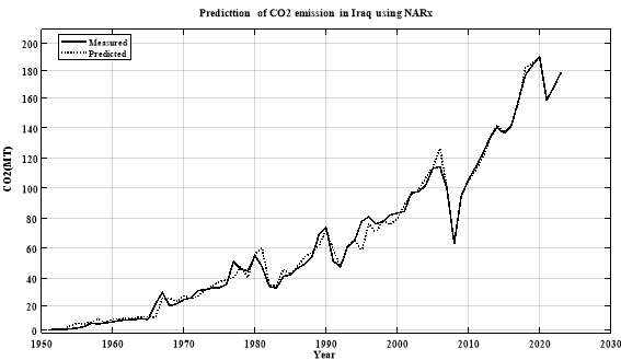
Fig. 11. The prediction of CO2 emission in Iraq using the ML-NARX model from 1950 to 2022

Considering the current CO ₂ emission forecast results for Iraq from 1950 to 2022, Table 3 shows the forecast results. The data indicates a state of increasing emissions rates and remaining at their highest levels for the coming years from 2023 to 2032, which means that the data will remain at the same level in the future. Considering the resulting data, the government and its local administrations should take the issue with a high level of interest and take serious measures to make a tangible change in the coming years to reduce emissions levels.

Table 4

Prediction of Iraq’s CO ₂ emission from 1950 to 2032

year	Prediction of CO 2 emission
2023	183128481.40
2024	190175702.20
2025	186897894.79
2026	186688572.79
2027	185516006.30
2028	184620123.10
2029	184746956.50
2030	184811601.03
2031	185113333.84
2032	184918443.44

Fig. 12 shows the forecast curve for the next ten years based on the results of the forecasts in Table 4 for the ML-NARX model. CO ₂ emissions will continue to increase while remaining at their highest levels. The forecast results have been combined with the historical database to draw the overall forecast curve in general from 1950 to 2032.

It can also be seen that the increase in CO ₂ emissions was 2.5446 million tons/year for the period from 1950 to 2022, i.e. the rate of increase reaches 8.62 %. As for what was predicted based on AI tools for the period from 2023 to 2032, the rate was 0.97 %, i.e. the rate of increase is 1.7820 million tons/year.

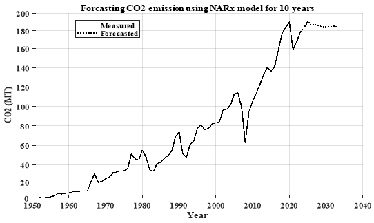
Fig. 12. The ML-NARX model for forecasting CO ₂ emissions

Hence, it is seen that looking at the zero value of CO ₂ emissions may be almost impossible under the current conditions of technological progress and aggressive climate policy, as it is not possible to specify a specific year for that, but if the percentage decreases significantly after 2032 or before by 1 % from 184 million tons/year, due to an improvement in energy efficiency, CO ₂ capture, reliance on renewable energy and reducing dependence on oil, then the estimate of zero CO ₂ emissions may take approximately until 2070 to 2080 to approach zero.

4. Comparison Results

This section discusses the performance of the proposed nerve network with the internal composition of the two hidden layers consisting of (10 25), and depending on the data of the carbon dioxide emissions for Iraq from the period (1950) to (2022) with the results of previous research that deal with the types of algorithms used and what their results provided, In light of the results that appeared to the performance of the performance (see table 5). This paper provided noticeable results that exceeded the results of the previous studies that I mentioned, as it achieved MSE (6.46E-04), which showed a superiority in the future prediction process for a period of ten years.

Table 5

Comparison of artificial intelligence models to predict CO2 emissions

REF/Year	Dataset/year	Adopted algorithm	MSE	MAE	RMSE
[40]/2024	2019 to 2022	GradBoost	NA	40.66	62.10
[41]/2024	1973 to 2022	L-RNN	135.5668592	NA	11.64331822
[42]/2023	1980 to 2019	LSTM	3676.646	45.524	60.635
[43]/2023	2017 to 2021	Catboost	3.83	2.41	1.9
[44]/2022	1972 to 2019	DNN	NA	5.820	8.099
[45]/2021	2003 to 2017	IMM	NA	NA	0.69

5. Conclusion

CO ₂ is the primary greenhouse gas responsible for global warming. CO ₂ has been designated as a greenhouse gas. It captures solar energy in the Earth's atmosphere that would have otherwise reflected away if the atmosphere were not contaminated with CO ₂ and other greenhouse gases. CO ₂ is the principal contributor to global warming and must be mitigated or diminished. Iraq entered the Paris Agreement to combat climate change and its adverse effects at COP21 in Paris on December 12, 2015. The accord became effective within a year and seeks to substantially diminish worldwide greenhouse gas emissions, aiming to restrict the global temperature rise this century to 2 degrees Celsius, while working to confine the increase to 1.5 degrees. The accord encompasses obligations to diminish CO ₂ emissions and try to adapt to the repercussions of climate change. Carbon capture and storage is a viable strategy for mitigating CO ₂ emissions. Nonetheless, it entails other inherent risks, including the likelihood of leakage, evaluation of economic, ecological, and social repercussions, and assessment of environmental disturbance intensity. This study seeks to identify a suitable forecasting model for CO ₂ emissions. The ML-NARX model was implemented to achieve the lowest MSE of 6.46E-04 and RMSE of 2.54E-02, using the permutation approach for the number of nodes in the two hidden layers while keeping other parameters constant. Consequently, we can ascertain that the (10 25) nodes framework of the nonlinear autoregressive time series model has shown superior efficacy in forecasting CO ₂ emissions in Iraq. The study's results indicate a robust link among the series. In light of the aforementioned findings, the Iraqi government and policymakers should proactively advance the energy industry and implement innovative ways to mitigate environmental pollution. These robust plans and policies should advocate for the consumption and production of alternative, cleaner, and renewable energy sources, such as wind, hydropower, solar, and bioenergy, rather than emphasizing the intensive combustion of non-renewable energy and its associated harmful fuels. Furthermore, policymakers in Iraq, along with governmental and local authorities, can utilize this research to assess the condition of the energy sector and mitigate the likelihood of various environmental difficulties and opportunities. This research demonstrates that substantial energy enhancements and restructuring are essential to elevate genuine economic growth and enhance environmental sustainability over time. Researchers are investigating the influence of various sectors and their share of overall CO ₂ emissions in Iraq, as well as forecasting sector-specific contributions.

Data Availability Statement

The data used for this study are publicly available and are reported in the paper.

Author Contributions

Data collection, H. A. S; Formal analysis, H. A. S; Investigation, R. M. H; Funding acquisition, M. A. H; Methodology, H. A. S; Software, R. M. H; Writing, H. A. S; Resources, M. A. H.

Abbreviations ARDL: autoregressive distributed lag; Catboost: categorical boosting; COP: crude oil production; CO ₂ : carbon dioxide; DNN: dense neural network; HDI: human development index; LSTM: long short term memory; MAE: mean absolute error; L-RNN: layer recurrent neural network; ML-NARX: multilayer nonlinear autoregressive exogenous; MSE: mean squared error; MPC: model predictive control; NAR: nonlinear Autoregressive; NARX: nonlinear autoregressive exogenous; NARDL: non-linear autoregressive distributed lag; IMM: Inclusive Multiple Model; R ² : regression; RMSE: root mean squared error; SARFIMA: seasonal autoregressive fractionally integrated moving average; VAR: vector autoregressive;

Conflicts of Interest

The authors declare no conflict of interest.

References:

1. Kabir, M., U. E. Habiba, W. Khan, A. Shah, S. Rahim, R. Patricio, L. Ali, and M. Shafiq, Climate change due to increasing concentration of carbon dioxide and its impacts on environment in 21st century; a mini review. Journal of King Saud University-Science, 2023. 35(5): p. 102693.
2. Nunes, L.J., The rising threat of atmospheric CO2: a review on the causes, impacts, and mitigation strategies. Environments, 2023. 10(4): p. 66.
3. Omri, A., B. Kahouli, H. Afi, and M. Kahia, Impact of environmental quality on health outcomes in Saudi Arabia: does research and development matter? Journal of the Knowledge Economy, 2023. 14(4): p. 4119–4144.
4. Abedin, B., M. R. Gabor, I. O. Susanu, and Y. F. Jaber, Exploring the Perspectives of Oil and Gas Industry Managers on the Adoption of Sustainable Practices: AQ Methodology Approach to Green Marketing Strategies. Sustainability, 2024. 16(14): p. 5948.
5. Yousif, B., O. El-joumayle, and J. Baban, Exploring the Water-Energy-Food nexus in context of conflict in Iraq. Energy Nexus, 2023. 11: p. 100233.
6. Awadh, S.M., Impact of North African sand and dust storms on the Middle East using Iraq as an example: Causes, sources, and mitigation. Atmosphere, 2023. 14(1): p. 180.
7. Amnuaylojaroen, T., Perspective on the Era of Global Boiling: A Future beyond Global Warming. Advances in Meteorology, 2023. 2023(1): p. 5580606.
8. Hassan, W.H., B. K. Nile, Z. K. Kadhim, K. Mahdi, M. Riksen, and R. F. Thiab, Trends, forecasting and adaptation strategies of climate change in the middle and west regions of Iraq. SN Applied Sciences, 2023. 5(12): p. 312.
9. Ganie, F.A., N. ud Wani, and M. Gani, Exposure to indoor household air pollution and its impact. Hazardous Chemicals, 2025: p. 765.
10. Arshad, K., N. Hussain, M. H. Ashraf, and M. Z. Saleem, Air pollution and climate change as grand challenges to sustainability. Science of The Total Environment, 2024: p. 172370.
11. Khurana, S., S. Saxena, S. Jain, and A. Dixit, Predictive modeling of engine emissions using machine learning: A review. Materials Today: Proceedings, 2021. 38: p. 280–284.
12. Sarker, I.H., Machine learning for intelligent data analysis and automation in cybersecurity: current and future prospects. Annals of Data Science, 2023. 10(6): p. 1473–1498.
13. Rehman, A., S. Naz, M. I. Razzak, F. Akram, and M. Imran, A deep learning-based framework for automatic brain tumors classification using transfer learning. Circuits, Systems, and Signal Processing, 2020. 39(2): p. 757–775.
14. Jumaah, H.J., M. H. Ameen, S. Mahmood, and S. J. Jumaah, Study of air contamination in Iraq using remotely sensed Data and GIS. Geocarto International, 2023. 38(1): p. 2178518.
15. Masini, R.P., M. C. Medeiros, and E. F. Mendes, Machine learning advances for time series forecasting. Journal of economic surveys, 2023. 37(1): p. 76–111.
16. Mustakim, R., M. Mamat, and H. T. Yew, Towards on-site implementation of multi-step air pollutant index prediction in Malaysia industrial area: Comparing the NARX neural network and support vector regression. Atmosphere, 2022. 13(11): p. 1787.
17. Bukhari, A.H., M. A. Z. Raja, M. Shoaib, and A. K. Kiani, Fractional order Lorenz based physics informed SARFIMA-NARX model to monitor and mitigate megacities air pollution. Chaos, Solitons & Fractals, 2022. 161: p. 112375.
18. Jung, H. and J. H. Lee, Flexible operation of Post-combustion CO2 capture process enabled by NARX-MPC using neural network. Computers & Chemical Engineering, 2023. 179: p. 108447.
19. Ma, D., J. Gao, Z. Gao, H. Jiang, Z. Zhang, and J. Xie, Gas leakage recognition for CO2 geological sequestration based on the time series neural network. Chinese Journal of Chemical Engineering, 2020. 28(9): p. 2343–2357.
20. Mutascu, M., CO2 emissions in the USA: new insights based on ANN approach. Environmental Science and Pollution Research, 2022. 29(45): p. 68332–68356.
21. Ahad, M., Quantile-based assessment of energy-CO2 emission nexus in Pakistan. Environmental Science and Pollution Research, 2024. 31(5): p. 7345–7363.
22. Sama, J. M. S., F. E. Sapnken, I. M. Mfetoum, and J. G. Tamba, The nexus between crude oil production, human development and economic growth in Cameroon (1977–2019). Energy Strategy Reviews, 2024. 52: p. 101341.
23. Our World in Data. Avialable: https://ourworldindata.org/grapher/annual-co-emissions-by-region. (Accessed on 9 October 2023).
24. Qader, M.R., S. Khan, M. Kamal, M. Usman, and M. Haseeb, Forecasting carbon emissions due to electricity power generation in Bahrain. Environmental Science and Pollution Research, 2021: p. 1–12.
25. Jankiewicz, M. and E. Szulc, Analysis of spatial effects in the relationship between CO2 emissions and renewable energy consumption in the context of economic growth. Energies, 2021. 14(18): p. 5829.
26. Falocchi, M., D. Zardi, and L. Giovannini, Meteorological normalization of NO2 concentrations in the Province of Bolzano (Italian Alps). Atmospheric Environment, 2021. 246: p. 118048.
27. Fang, W., R. Zhu, and J. C.-W. Lin, An air quality prediction model based on improved Vanilla LSTM with multichannel input and multiroute output. Expert systems with applications, 2023. 211: p. 118422.
28. Platt, J.A., S. G. Penny, T. A. Smith, T.-C. Chen, and H. D. Abarbanel, A systematic exploration of reservoir computing for forecasting complex spatiotemporal dynamics. Neural Networks, 2022. 153: p. 530–552.
29. Passalis, N., A. Tefas, J. Kanniainen, M. Gabbouj, and A. Iosifidis, Deep adaptive input normalization for time series forecasting. IEEE transactions on neural networks and learning systems, 2019. 31(9): p. 3760–3765.
30. Lee, C., D. E. Jung, D. Lee, K. H. Kim, and S. L. Do, Prediction performance analysis of artificial neural network model by input variable combination for residential heating loads. Energies, 2021. 14(3): p. 756.
31. Cheng, A. and Y. M. Low, Improved generalization of NARX neural networks for enhanced metamodeling of nonlinear dynamic systems under stochastic excitations. Mechanical Systems and Signal Processing, 2023. 200: p. 110543.
32. Sansa, I., Z. Boussaada, and N. M. Bellaaj, Solar radiation prediction using a novel hybrid model of ARMA and NARX. Energies, 2021. 14(21): p. 6920.
33. Ramadevi, B. and K. Bingi, Chaotic time series forecasting approaches using machine learning techniques: A review. Symmetry, 2022. 14(5): p. 955.
34. Amirkhani, S., A. Tootchi, and A. Chaibakhsh, Fault detection and isolation of gas turbine using series–parallel NARX model. ISA transactions, 2022. 120: p. 205–221.
35. AL-Rousan, N. and H. Al-Najjar, A comparative assessment of time series forecasting using NARX and SARIMA to predict hourly, daily, and monthly global solar radiation based on short-term dataset. Arabian Journal for Science and Engineering, 2021. 46(9): p. 8827–8848.
36. Serikov, T., A. Zhetpisbayeva, S. Mirzakulova, K. Zhetpisbayev, Z. Ibrayeva, A. Tolegenova, L. Soboleva, and B. Zhumazhanov, Application of the NARX neural network for predicting a one-dimensional time series. Eastern-European Journal of Enterprise Technologies, 2021. 5(4): p. 113.
37. Khan, N.A., M. Sulaiman, C. A. Tavera Romero, and F. K. Alarfaj, Theoretical analysis on absorption of carbon dioxide (CO2) into solutions of phenyl glycidyl ether (PGE) using nonlinear autoregressive exogenous neural networks. Molecules, 2021. 26(19): p. 6041.
38. Di Nunno, F. and F. Granata, Groundwater level prediction in Apulia region (Southern Italy) using NARX neural network. Environmental Research, 2020. 190: p. 110062.
39. Sameer, H.A., S. K. Gharghan, and A. H. Mutlag, Hybridization of particle swarm optimization algorithm with neural network for COVID‐19 using computerized tomography scan and clinical parameters. The Journal of Engineering, 2023. 2023(2): p. e12226.
40. Ostermann, A., A. Bajrami, and A. Bogensperger, Short-term forecasting of German generation-based CO2 emission factors using parametric and non-parametric time series models. Energy Informatics, 2024. 7(1): p. 2.
41. Chukwunonso, B.P., I. Al-Wesabi, L. Shixiang, K. AlSharabi, A. A. Al-Shamma’a, H. M. H. Farh, F. Saeed, T. Kandil, and A. M. Al-Shaalan, Predicting carbon dioxide emissions in the United States of America using machine learning algorithms. Environmental Science and Pollution Research, 2024. 31(23): p. 33685–33707.
42. Kumari, S. and S. K. Singh, Machine learning-based time series models for effective CO2 emission prediction in India. Environmental Science and Pollution Research, 2023. 30(55): p. 116601–116616.
43. Natarajan, Y., G. Wadhwa, K. Sri Preethaa, and A. Paul, Forecasting carbon dioxide emissions of light-duty vehicles with different machine learning algorithms. Electronics, 2023. 12(10): p. 2288.
44. Faruque, M.O., M. A. J. Rabby, M. A. Hossain, M. R. Islam, M. M. U. Rashid, and S. Muyeen, A comparative analysis to forecast carbon dioxide emissions. Energy Reports, 2022. 8: p. 8046–8060.
45. Shabani, E., B. Hayati, E. Pishbahar, M. A. Ghorbani, and M. Ghahremanzadeh, A novel approach to predict CO2 emission in the agriculture sector of Iran based on Inclusive Multiple Model. Journal of Cleaner Production, 2021. 279: p. 123708.