


Gravity Model of trade has already for decades been the most popular theory to explain trade flows between nations. The theory matched very well with the empiric observations, so it became a common tool among economists, even though it lacked thorough theoretical justification. On the 21st century researchers have been able to provide us with solid theoretical backing for the Gravity Model of Trade. Regardless of all the existing and widely accepted modifications of the gravity model, one should always be careful in choosing a suitable version for his own study. Trade flows between different countries differ enormously and there isn’t a single specific model that would be the best possible option for all countries in the world.
Gravity model was first discovered in physics, when Newton in 1678 year, found out, that any two bodies in the universe attract each other with a force that is directly proportional to the product of their masses and inversely proportional to the square of the distance between them:

Where,
 — attractive force;
 and
and  — the masses of objects i and j correspondingly;
 — distance between the two objects;
G- gravitational constant.
In 1962 Jan Tinbergen proposed that roughly the same functional form could be applied to international trade flows. However, it has since been applied to a whole range of what we might call “social interactions” including migration, tourism, and foreign direct investment. This general gravity law for social interaction may be expressed in roughly the same notation.
Tinbergen began its analysis with the use of only three independent variables: GDP of the exporting country, the importing country's GDP and geographical distance between countries. The main form of Tinbergen gravity model is as follows:

In our research we will study Belarusian exports to its 10 most important trading partners between 2000 and 2012 years using the Gravity model of trade. Data are taken from public sources such as UN COMTRADE, CEPII, World Bank. We selected 10 countries represent roughly 80 % of Belarusian trade. Table 1 represents ten main trading partners of Belarus and its share in turnover.
Table 1
|
Main Trading Partners |
Share, % |
|
Russia |
49.6 |
|
Ukraine |
7.8 |
|
Germany |
6.0 |
|
Netherlands |
4.8 |
|
China |
4.2 |
|
Poland |
3.1 |
|
Italy |
2.5 |
|
Lithuania |
2.1 |
|
United Kingdom |
1.6 |
|
Kazakhstan |
1.2 |
(Source: National Statistics Committee of the Republic of Belarus)
I study Belarusian exports to its main trading partners using following function for export:

Where,
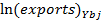 — Natural logarithm for Belarusian exports in country j in Y year.
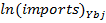 — Natural logarithm for imports in Belarus from country j in Y year.
 — Natural logarithm for Gross Domestic Product in Belarus in Y year.
 — Natural logarithm for Gross Domestic Product in country j in Y year.
 — Natural logarithm for population in Belarus in Y year.
 — Natural logarithm for population in country j in Y year.
 — Natural logarithm for distance from Belarus to country j in Y year.
 — Dummy variable for common boarder.
 — Dummy variable for former Soviet Union countries.
 — Parameter values.
Variables used:
1) Exports: for total annual export from Belarus to each country partner used the data collected from United Nations Commodity Trade Statistics Database. Exports calculated in FOB prices.
2) Imports: for total annual imports in Belarus from each country partner used the data collected from United Nations Commodity Trade Statistics Database. Imports calculated in CIF prices.
3) GDP: for annual GDP values data was taken from World Bank world development indicators dataset. All the GDP values were gross values for the whole country and they were counted in US dollars, which made them easily comparable. GDP is a measure of the size of country’s economy, so countries with high GDP values are assumed to trade more with each other than countries with low GDP values. GDP calculated in current US dollars.
4) Population: The populations of all countries were found from World Bank world development indicators dataset. Population is another time variant variable that should be positively correlated with trade as larger markets should develop larger trade flows with each other. On the other hand, a large economy is able to produce a wider variety of goods, so in a simplistic world, such a nation should have less need for foreign imports.
5) Distance: Distance is a time invariant variable, so it remains constant during the whole period of study. In Gravity Model of Trade distance is often used as a proxy for transaction costs for the trade between the two countries. Therefore a longer distance between two countries should reduce the amount of trade between them, as trade costs are assumed to rise. Recently it has been pointed out that a better approximation for the transportation costs could be received by applying also some infrastructure index, since a good infrastructure makes transportation cheaper and vice versa (Martinez-Zarzoso, Nowak-Lehmann, 2003). In this study still using only simple geographical distance, this should give good enough estimations for this study. Geodesic distances are calculated following the great circle formula, which uses latitudes and longitudes of the geographic coordinates of the capital cities.
6) Common border dummy variable: a dummy variable (time invariant variable) for countries that share a common border with Belarus. Neighboring countries would trade more, as the transportations costs should be relative low.
7) Former Soviet Union dummy variable: a dummy for countries that used to be part of Soviet Union. Formed Soviet Union republics were quite specialized in producing certain kind of goods, which were then centrally directed to other regions where such a good was needed. It have interested whether former Soviet republics still trade much with Belarus, or have they diversified its trade patterns and now trade equally with all countries.
Hausman test allows a choice between fixed effects (FE) and random effects (RE) models.
This test is based on the difference between the two estimates:  , where
  estimate obtained for the fixed effects model (it is consistent in the case of main and in the case of the alternative hypothesis),
 estimate obtained for the random effects model (it is consistent only in the case of main hypothesis).
Provided Hausman text using RE estimation from export presented below, we obtained results presented in figure 1:
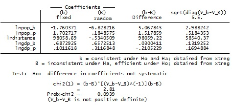
Fig. 1 Hausman test estimation
Since p-value > 0.01, the main hypothesis is not rejected.
The obtained results allow us to conclude that in our case fits the model with random individual effects. This should be expected, since the study was chosen specific country set, their composition has not changed from year to year. Same situation is for imports.
Hausman test is carried out only with the estimates of the coefficients that are present simultaneously in the regressions and FE, and RE. This means that it only takes into account the coefficients are not time-invariant regressor.
In this study we used panel data method and perform the regressions with Stata-program. Apply the random effects (RE) techniques. We also control Multilateral resistance term by construction year and country dummies.
Results for exports presented in table 4.3:
Random-effects GLS regression Number of obs = 130
Group variable: pairid Number of groups = 10
R-sq: within = 0.7337 Obs per group: min = 13
Between = 1.0000 avg = 13.0
overall = 0.8973 max = 13
Wald chi2(9) =.
corr(u_i, X) = 0 (assumed) Prob > chi2 =.
Table 2
(Std. Err. adjusted for 10 clusters in pairid)
|
lnexport |
Coeff. |
RobustStd. Err. |
z |
P>|z| |
[95 % Conf. Interval] |
|
|
Lngdp_b |
3.542536 |
1.659641 |
2.13 |
0.033 |
0.2896992 |
6.795373 |
|
lngdp_p |
-.1458501 |
0.5127144 |
-0.28 |
0.776 |
-1.150752 |
0.8590517 |
|
lnpop_b |
5.855042 |
2.698223 |
-2.17 |
0.030 |
-11.14346 |
-.5666231 |
|
lnpop_p |
1.999553 |
0.7137957 |
2.80 |
0.005 |
.6005387 |
3.398567 |
|
lndistance |
-0.1815647 |
1.367548 |
-0.13 |
0.894 |
-2.86191 |
2.498781 |
|
boarderdum |
-2.764532 |
1.420592 |
-1.95 |
0.052 |
-5.548841 |
0.0197768 |
|
sovietdum |
-.1235377 |
0.7282934 |
-0.17 |
-1.550966 |
-1.550966 |
1.303891 |
|
sigma_u sigma_e rho |
0 0.46219294 0 (fraction of variance due to u_i) |
|||||
We can see a number of interesting features apparent from these random effects estimation for export from Belarus to a country partner. The first is that equation fits the data relatively well: its overall R2 is 0.89 for, which means that the explanatory variables account for over 89 per cent of the observed variation in trade in the data for exports. To interpret the model results further, we need to look more closely at the estimated coefficients and their corresponding t-tests.
Population in Belarus: -5.855042, fits in 95 % confidence interval and statistically significant at 5 per cent level. What means that growth of Belarusian population in 1 % tends to reduce exports from Belarus by 5.86 %. This results conflict with intuition and will be explained below, in conclusion.
Population in country partner have positive sign and coefficient value is 1.999553, that means that 1 % growth in population in country partner tends to increase trade by about 2 per cent, and this effects statistically significant at the 1 per cent level (indicated by a p-value in the fifth column of less than 0.01).
As was expected distance coefficient have a negative sign value is -0.1815647, but it looks statistically insignificant, that means that’s distance don’t have a great influence on Belarusian exports. This estimation also conflict with intuition and will be explained below.
GDP of Belarus coefficient value have positive sign and meaning is 3.542536, that means that 1 % growth in GDP in Belarus tends to increase exports to country partner by about 3.54 per cent, and this effect is statistically significant at the 5 per cent level.
GDP of country partner unexpected have a negative sign and statistically insignificant, That mean GDP in country partner don’t have a great influence on Belarusian exports in main ten country partners.
Note, however, that while the coefficients for the natural logarithm of continuous variables (e.g. GDP, distance) are elasticity, the coefficients for the dummies (such as a dummy denoting whether two countries share same boarder) are not. They need to be transformed as follows in order to be interpreted as elasticity: elasticity = exp(a)–1 where a is the estimated coefficient of the dummy variable and exp(a) is exponential.
Common Border Dummy Variable value is -2.764532, that means that common boarder tends to reduce Belarusian exports by about -0.94 per cent, and this effect is statistically significant at 10 per cent level.
Former Soviet Union dummy value is -0.1235377, but this effect is statistically insignificant. Common soviet history doesn’t have significant influence on Belarusian exports to country partner.
When Belarusian exports to its main trading partners were studied, several conclusions could be made. First of all, the export structure of Belarus differs a lot from that of an average industrialized country. Therefore also the results of this study differed from those that are usually gotten from gravity model studies of industrialized countries. Majority of Belarusian exports are raw materials, oil products, potassium fertilizers.
Secondly, the distance between Belarus and its trading partners doesn’t really affect the Belarusian exports, whereas for an average industrialized country a long distance to a trading partner tends to decrease trade significantly. A likely explanation for also this result could be the export structure of Belarus. Raw material markets are global and some of them have to be exported very long distances, as they can be produced in only certain locations.
Also the population of the export market seems to be a bad variable to explain Belarusian exports. Once again, the demand for raw materials doesn’t depend on the size of population, but it does seem to depend on the wealth of the nation. According to this study the wealth (GDP size) of a country seems to explain some of the demand for Belarusian exports and especially the demand for oil products exports. This result matches with the intuition, as a wealthy country has typically higher need for raw materials, gasoline and energy than a less developed country has.
There is also a strong negative correlation between Belarusian population and Belarusian exports, but there is still no reason to believe that a decline in Belarusian population would cause increase in Belarusian exports. This relationship seems to be rather just a coincidence. Belarusian population declined on average during the period studied, while the Belarusian exports increase rapidly.
