


Factor analysis is a statistical method used to describe variability among observed, correlated variables in terms of a potentially lower number of unobserved variables called factors. For example, it is possible that variations in say six observed variables mainly reflect the variations in two unobserved (underlying) variables. Factor analysis searches for such joint variations in response to unobserved latent variables. The observed variables are modeled as linear combinations of the potential factors, plus «error» terms. The information gained about the interdependencies between observed variables can be used later to reduce the set of variables in a dataset. Factor analysis originated in psychometrics and is used in behavioral sciences, social sciences, marketing, product management, operations research, and other fields that deal with data sets where there are large numbers of observed variables that are thought to reflect a smaller number of underlying/latent variables.
Factor analysis was invented nearly 100 years ago by psychologist Charles Spearman, who hypothesized that the enormous variety of tests of mental ability--measures of mathematical skill, vocabulary, other verbal skills, artistic skills, logical reasoning ability, etc.--could all be explained by one underlying «factor» of general intelligence that he called g. He hypothesized that if g could be measured and you could select a subpopulation of people with the same score on g, in that subpopulation you would find no correlations among any tests of mental ability. In other words, he hypothesized that g was the only factor common to all those measures.
It was an interesting idea, but it turned out to be wrong. Today the College Board testing service operates a system based on the idea that there are at least three important factors of mental ability--verbal, mathematical, and logical abilities--and most psychologists agree that many other factors could be identified as well.
The factor analysis model
In the factor analysis model, the measured variables depend on a smaller number of unobserved (latent) factors. Because each factor may affect several variables in common, they are known as «common factors». Each variable is assumed to depend on a linear combination of the common factors, and the coefficients are known as loadings. Each measured variable also includes a component due to independent random variability, known as «specific variance» because it is specific to one variable.
Specifically, factor analysis assumes that the covariance matrix of your data is of the form
SigmaX = Lambda*Lambda' + Psi
where Lambda is the matrix of loadings, and the elements of the diagonal matrix Psi are the specific variances. The function factoran fits the factor analysis model using maximum likelihood.
Factor Analysis from a Covariance/Correlation Matrix
You made the fits above using the raw test scores, but sometimes you might only have a sample covariance matrix that summarizes your data. factoran accepts either a covariance or correlation matrix, using the 'Xtype' parameter, and gives an identical result to that from the raw data.
Sigma = cov(grades);
[LoadingsCov,specVarCov] = ...
factoran(Sigma,2,'Xtype','cov','rotate','none');
LoadingsCov
LoadingsCov =
0.6289 0.3485
0.6992 0.3287
0.7785 -0.2069
0.7246 -0.2070
0.8963 -0.0473
Matrix Decomposition and Rank
This optional section gives a little more detail on the mathematics of factor analysis. I assume you are familiar with the central theorem of analysis of variance: that the sum of squares of a dependent variable Y can be partitioned into components which sum to the total. In any analysis of variance the total sum of squares can be partitioned into model and residual components. In a two-way factorial analysis of variance with equal cell frequencies, the model sum of squares can be further partitioned into row, column, and interaction components.
The central theorem of factor analysis is that you can do something similar for an entire covariance matrix. A covariance matrix R can be partitioned into a common portion C which is explained by a set of factors, and a unique portion U unexplained by those factors. In matrix terminology, R = C + U, which means that each entry in matrix R is the sum of the corresponding entries in matrices C and U.
As in analysis of variance with equal cell frequencies, the explained component C can be broken down further. C can be decomposed into component matrices c1, c2, etc., explained by individual factors. Each of these one-factor components cj equals the «outer product» of a column of «factor loadings». The outer product of a column of numbers is the square matrix formed by letting entry jk in the matrix equal the product of entries j and k in the column. Thus if a column has entries.9,.8,.7,.6,.5, as in the earlier example, its outer product is
.81 .72 .63 .54 .45
.72 .64 .56 .48 .40
c1 .63 .56 .49 .42 .35
.54 .48 .42 .36 .30
.45 .40 .35 .30 .25
Earlier I mentioned the off-diagonal entries in this matrix but not the diagonal entries. Each diagonal entry in a cj matrix is actually the amount of variance in the corresponding variable explained by that factor. In our example, g correlates.9 with the first observed variable, so the amount of explained variance in that variable is.92 or.81, the first diagonal entry in this matrix.
In the example there is only one common factor, so matrix C for this example (denoted C55) is C55 = c1. Therefore the residual matrix U for this example (denoted U55) is U55 = R55 — c1. This gives the following matrix for U55:
.19 .00 .00 .00 .00
.00 .36 .00 .00 .00
U55 .00 .00 .51 .00 .00
.00 .00 .00 .64 .00
.00 .00 .00 .00 .75
This is the covariance matrix of the portions of the variables unexplained by the factor. As mentioned earlier, all off-diagonal entries in U55 are 0, and the diagonal entries are the amounts of unexplained or unique variance in each variable.
Often C is the sum of several matrices cj, not just one as in this example. The number of c-matrices which sum to C is the rank of matrix C; in this example the rank of C is 1. The rank of C is the number of common factors in that model. If you specify a certain number m of factors, a factor analysis program then derives two matrices C and U which sum to the original correlation or covariance matrix R, making the rank of C equal m. The larger you set m, the closer C will approximate R. If you set m = p, where p is the number of variables in the matrix, then every entry in C will exactly equal the corresponding entry in R, leaving U as a matrix of zeros. The idea is to see how low you can set m and still have C provide a reasonable approximation to R.
The number of factors.
The first uses a formal significance test to identify the number of common factors. Let N denote the sample size, p the number of variables, and m the number of factors. Also RU denotes the residual matrix U transformed into a correlation matrix, |RU| is its determinant, and ln(1/|RU|) is the natural logarithm of the reciprocal of that determinant.
To apply this rule, first compute G = N-1-(2p+5)/6-(2/3)m. Then compute
Chi-square = G ln(1/|RU|)
with
df =.5 [(p-m)2-p-m]
If it is difficult to compute ln(1/|RU|), that expression is often well approximated by rU2, where the summation denotes the sum of all squared correlations above the diagonal in matrix RU.
To use this formula to choose the number of factors, start with m = 1 (or even with m = 0) and compute this test for successively increasing values of m, stopping when you find nonsignificance; that value of m is the smallest value of m that is not significantly contradicted by the data. The major difficulty with this rule is that in my experience, with moderately large samples it leads to more factors than can successfully be interpreted.
Factor Analysis from a Covariance/Correlation Matrix
You made the fits above using the raw test scores, but sometimes you might only have a sample covariance matrix that summarizes your data. factoran accepts either a covariance or correlation matrix, using the 'Xtype' parameter, and gives an identical result to that from the raw data.
Sigma = cov(grades);
[LoadingsCov,specVarCov] = ...
factoran(Sigma,2,'Xtype','cov','rotate','none');
LoadingsCov
LoadingsCov =
0.6289 0.3485
0.6992 0.3287
0.7785 -0.2069
0.7246 -0.2070
0.8963 -0.0473
Factor Rotation
Sometimes, the estimated loadings from a factor analysis model can give a large weight on several factors for some of the measured variables, making it difficult to interpret what those factors represent. The goal of factor rotation is to find a solution for which each variable has only a small number of large loadings, i.e., is affected by a small number of factors, preferably only one.
If you think of each row of the loadings matrix as coordinates of a point in M-dimensional space, then each factor corresponds to a coordinate axis. Factor rotation is equivalent to rotating those axes, and computing new loadings in the rotated coordinate system. There are various ways to do this. Some methods leave the axes orthogonal, while others are oblique methods that change the angles between them.
Varimax is one common criterion for orthogonal rotation.factoranperforms varimax rotation by default, so you do not need to ask for it explicitly.
[LoadingsVM,specVarVM,rotationVM] = factoran(grades,2);
A quick check of the varimax rotation matrix returned byfactoranconfirms that it is orthogonal. Varimax, in effect, rotates the factor axes in the figure above, but keeps them at right angles.
rotationVM'*rotationVM
ans =
1.0000 -0.0000
-0.0000 1.0000
A biplot of the five variables on the rotated factors shows the effect of varimax rotation.
biplot(LoadingsVM, 'varlabels',num2str((1:5)'));
title('Varimax Solution');
xlabel('Latent Factor 1'); ylabel('Latent Factor 2');
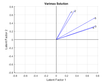
Varimax has rigidly rotated the axes in an attempt to make all of the loadings close to zero or one. The first two exams are closest to the second factor axis, while the third and fourth are closest to the first axis and the fifth exam is at an intermediate position. These two rotated factors can probably be best interpreted as «quantitative ability» and «qualitative ability». However, because none of the variables are near a factor axis, the biplot shows that orthogonal rotation has not succeeded in providing a simple set of factors.
Because the orthogonal rotation was not entirely satisfactory, you can try using promax, a common oblique rotation criterion.
[LoadingsPM,specVarPM,rotationPM] = ...
factoran(grades,2,'rotate','promax');
A check on the promax rotation matrix returned byfactoranshows that it is not orthogonal. Promax, in effect, rotates the factor axes in the first figure separately, allowing them to have an oblique angle between them.
rotationPM'*rotationPM
ans =
1.9405 -1.3509
-1.3509 1.9405
A biplot of the variables on the new rotated factors shows the effect of promax rotation.
biplot(LoadingsPM, 'varlabels',num2str((1:5)'));
title('Promax Solution');
xlabel('Latent Factor 1'); ylabel('Latent Factor 2');
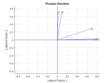
Promax has performed a non-rigid rotation of the axes, and has done a much better job than varimax at creating a «simple structure». The first two exams are close to the second factor axis, while the third and fourth are close to the first axis, and the fifth exam is in an intermediate position. This makes an interpretation of these rotated factors as «quantitative ability» and «qualitative ability» more precise.
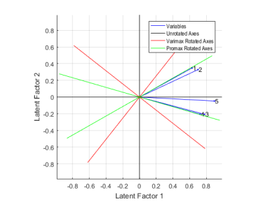
Instead of plotting the variables on the different sets of rotated axes, it's possible to overlay the rotated axes on an unrotated biplot to get a better idea of how the rotated and unrotated solutions are related.
h1 = biplot(Loadings2, 'varlabels',num2str((1:5)'));
xlabel('Latent Factor 1'); ylabel('Latent Factor 2');
hold on
invRotVM = inv(rotationVM);
h2 = line([-invRotVM(1,1) invRotVM(1,1) NaN -invRotVM(2,1) invRotVM(2,1)], ...
[-invRotVM(1,2) invRotVM(1,2) NaN -invRotVM(2,2) invRotVM(2,2)],'Color',[1 0 0]);
invRotPM = inv(rotationPM);
h3 = line([-invRotPM(1,1) invRotPM(1,1) NaN -invRotPM(2,1) invRotPM(2,1)], ...
[-invRotPM(1,2) invRotPM(1,2) NaN -invRotPM(2,2) invRotPM(2,2)],'Color',[0 1 0]);
hold off
axis square
lgndHandles = [h1(1) h1(end) h2 h3];
lgndLabels = {'Variables','Unrotated Axes','Varimax Rotated Axes','Promax Rotated Axes'};
legend(lgndHandles, lgndLabels, 'location','northeast', 'fontname','arial narrow');
Factor analysis is a way to fit a model to multivariate data to estimate just this sort of interdependence.
Multivariate data often include a large number of measured variables, and sometimes those variables «overlap» in the sense that groups of them may be dependent.
References:
- Darlington, Richard B., Sharon Weinberg, and Herbert Walberg (1973). Canonical variate analysis and related techniques. Review of Educational Research, 453–454.
- Gorsuch, Richard L. (1983) Factor Analysis. Hillsdale, NJ: Erlbaum
- Morrison, Donald F. (1990) Multivariate Statistical Methods. New York: McGraw-Hill.
- Rubenstein, Amy S. (1986). An item-level analysis of questionnaire-type measures of intellectual curiosity. Cornell University Ph. D. thesis.
