


1. Introduction
We consider numerical solving the hyperbolic equation
![]()
equipped with suitable initial and boundary conditions for known velocity coefficient ![]()
Among the successful numerical methods for solving this equation we mention such nonoscillatory conservative finite difference shemes as TVD (total variation diminishing), TVB (total variation bounded), ENO (essentially nonoscillatory), and CABARET (Compact Accurate Boundary Adjusting high REsolution Technique) shemes (see [1]- [11] and the reference there). This approach uses the traditional difference approximation of temporal derivative and is liable to Courant — Friedrichs — Lewy (CFL) condition for ratio between steps in time and space.
The other approach focuses on the approximation of the whole operator of problem (1) as the partial derivative in some direction of the space ![]() This approach is developed under different names: methods of trajectories or modified characteristics and semi-Lagrangian one (see, for example, [12]- [19] and the reference there).
This approach is developed under different names: methods of trajectories or modified characteristics and semi-Lagrangian one (see, for example, [12]- [19] and the reference there).
In order to highlight the essential ingredients of suggested approach we shall operate with one-dimensional problem again, keeping in mind that we shall extend this method in subsequent papers. In this paper, we will first show how to consider the possible boundary conditions in contrast to the periodic conditions of the previous paper [16]. Then we modify the presented algorithm for big and huge velocity and give a numerical example that demonstrates the stability independent of CFL condition.
2. The statement of problem and the main theorem
So, in the rectangle ![]() consider equation
consider equation
![]() (1)
(1)
Assume that coefficient ![]() is given at
is given at ![]() and is positive for simplicity sake.
and is positive for simplicity sake.
Unknown function ![]() satisfies the initial condition
satisfies the initial condition
![]() (2)
(2)
and boundary condition
![]() (3)
(3)
Assuming the continuity of ![]() at
at ![]() we get
we get ![]() at the coordinate origin. Moreover, for continuity of first partial derivatives in (1) the following equality must hold:
at the coordinate origin. Moreover, for continuity of first partial derivatives in (1) the following equality must hold:
![]()
By simple calculations we can obtain the necessary condition for the continuity of the second partial derivatives at the point (0, 0), etc. We will not dwell on the question of the sufficiency of this conditions for the smoothness of the solution ![]() and at once we assume sufficient smoothness of the velocity
and at once we assume sufficient smoothness of the velocity ![]() and solution
and solution ![]() for further considerations.
for further considerations.
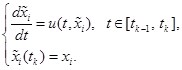
Let us take two time lines ![]() with
with ![]() and two nodes
and two nodes ![]()
For both these nodes we construct the characteristics ![]() of equation (1) at segment
of equation (1) at segment ![]() [20, 21]. They satisfy the ordinary differential equation with different initial values:
[20, 21]. They satisfy the ordinary differential equation with different initial values:
 (4)
(4)
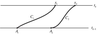
Fig. 1. Trajectories in standard (first) situation
These characteristics define two trajectories ![]() in plane
in plane ![]() when
when ![]() The typical situation is considered in the previous paper [20] when each of these trajectories crosses line
The typical situation is considered in the previous paper [20] when each of these trajectories crosses line ![]() in some point
in some point ![]() We supposed that they are not mutually crossed and therefore
We supposed that they are not mutually crossed and therefore ![]() For this case the following result was proved in [16].
For this case the following result was proved in [16].
Theorem 1. For smooth solution of equation (1) in the standard (first) situation (Fig. 1) we have equality
![]() (5)
(5)
But the boundary condition (3) may produce two other situations. First, for small ![]() the trajectory
the trajectory ![]() may be interrupted at line
may be interrupted at line ![]() at point
at point ![]() because function
because function ![]() is unknown for
is unknown for ![]() But trajectory
But trajectory ![]() continues up to line
continues up to line ![]() (see Fig. 2). And second, both trajectories
(see Fig. 2). And second, both trajectories ![]() and
and ![]() are interrupted at line
are interrupted at line ![]() at points
at points ![]() and
and ![]() (see Fig. 3). We enumerate these situations from one to three.
(see Fig. 3). We enumerate these situations from one to three.
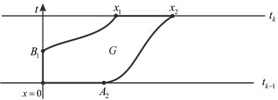
Fig. 2. Second situation: trajectory C1 is interrupted and C2 does not
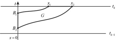
Fig. 3. Third situation: both trajectories C1 and C2 are interrupted
For last situations we prove two equalities.
Theorem 2. For smooth solution of equation (1) with boundary condition (3) in the second situation (Fig. 2) we get the equality
![]() (6)
(6)
Proof. Define by ![]() the curvilinear pentagon bounded by lines
the curvilinear pentagon bounded by lines ![]() And define by
And define by ![]() the corresponding parts of these lines, which form the boundary
the corresponding parts of these lines, which form the boundary ![]() (see Fig. 4). Introduce also the external normal
(see Fig. 4). Introduce also the external normal ![]() defined at each part of boundary except 5 vertices of pentagon.
defined at each part of boundary except 5 vertices of pentagon.
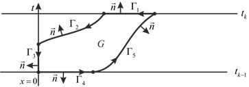
Fig. 4. Integration along the boundary in second case
Now use formula by Gauss-Ostrogradskii [20, 21] in the following form:
![]() (7)
(7)
where sing ![]() means scalar product. Since the boundary
means scalar product. Since the boundary ![]() consists of five parts we calculate the integral over
consists of five parts we calculate the integral over ![]() separately on each line:
separately on each line:
 (8)
(8)
Along the line ![]() the external normal equals
the external normal equals ![]() Then
Then
![]() (9)
(9)
At arbitrary point ![]() the tangent vector is
the tangent vector is ![]() Therefore the external normal (that is orthogonal to it) equals
Therefore the external normal (that is orthogonal to it) equals
![]() (10)
(10)
It implies equality
![]() (11)
(11)
Along the line ![]() the external normal equals
the external normal equals ![]() Then
Then
![]() (12)
(12)
For other two parts of the boundary we use the same way to calculate the integrals:
![]() (13)
(13)
![]() (14)
(14)
Combination of (7) — (9) and (11) — (14) implies (6):
![]() ?
?
The next result is justificated like previous theorem with some simplification. Therefore we give it without any proof.
Theorem 3. For smooth solution of equation (1) with boundary condition (3) in the third situation (Fig. 3) we get the equality
![]() (15)
(15)
Note that this situation contains the case when ![]() and
and ![]() coincides with
coincides with ![]()
So, consideration of the boundary conditions in the calculation expressions ![]() resulted in an additional calculation of the integrals along
resulted in an additional calculation of the integrals along ![]() of known function
of known function ![]() In this sense, consideration of boundary conditions makes minor modifications into the algorithms discussed below, so in further considerations we return to the periodic case.
In this sense, consideration of boundary conditions makes minor modifications into the algorithms discussed below, so in further considerations we return to the periodic case.
3. Piece-wise linear discrete approximation
So, let the condition of periodicity holds for the problem (1) — (2), namely functions ![]() are supposed periodical in
are supposed periodical in ![]() with period
with period ![]() and are smooth enough for further considerations.
and are smooth enough for further considerations.
Now we formulate some modification of numerical algorithm from [16] for solving problem (1) — (2). First, take integer ![]() and construct uniform mesh in
and construct uniform mesh in ![]() with nodes
with nodes ![]() and meshsize
and meshsize ![]() Than take integer
Than take integer ![]() and construct uniform mesh in
and construct uniform mesh in ![]() with nodes
with nodes ![]() and meshsize
and meshsize ![]() Then make the following cycle for
Then make the following cycle for ![]() supposing that the approximate solution
supposing that the approximate solution ![]() is known yet at previous time-level for
is known yet at previous time-level for ![]()
1. With the help of values in these points and periodicity we construct the piecewise linear (periodical) interpolant
![]() (16)
(16)
2. For each point ![]() construct approximate trajectories
construct approximate trajectories ![]() down to time-level
down to time-level ![]() for example, by Runge-Kutta method. They produce cross-points
for example, by Runge-Kutta method. They produce cross-points ![]() If
If ![]() goes outside segment
goes outside segment ![]() we use periodicity of our data. One can see that we get values
we use periodicity of our data. One can see that we get values ![]() which do not coincide with exact values
which do not coincide with exact values ![]() Let we solve equations (4) with the following accuracy:
Let we solve equations (4) with the following accuracy:
![]() (17)
(17)
where ![]() is small enough.
is small enough.
3. For each interval ![]() compute integral
compute integral
![]() (18)
(18)
by trapezoid quadrature formula separately at each nonempty subinterval ![]() where
where ![]() is linear.
is linear.
4. Due to Theorem 1 it is supposed that
![]() (19)
(19)
Finally we put
![]() (20)
(20)
Thus, we complete our cycle which may be repeated up to last time-level ![]()
Condensed form of this algorithm in terms of piecewise linear periodical interpolants is written as follows:
![]() (21)
(21)
So, we get approximate discrete solution ![]() at each time-level
at each time-level ![]() First we prove the conservation law in discrete form.
First we prove the conservation law in discrete form.
Let a discrete function ![]() is given, and we construct piecewise linear interpolant
is given, and we construct piecewise linear interpolant ![]() with period 1.
with period 1.
Theorem 4. For any initial condition ![]() the approximate solution (16) — (20)
the approximate solution (16) — (20) ![]() satisfies the equality:
satisfies the equality:
![]() (22)
(22)
Proof. The justification directly coincides with the proof of Theorem 2 in [16] with substitution ![]() instead of
instead of ![]()
It is interesting that this discrete conservation law is exactly valid for an approximate values ![]()
Now we prove a stability of algorithm (17) — (20) in the discrete norm analogous to that of space ![]()
![]() (23)
(23)
Theorem 5. For any intermediate discrete function ![]() the solution
the solution ![]() of (17) — (20) satisfies the inequality:
of (17) — (20) satisfies the inequality:
![]() (24)
(24)
Proof. Again the justification directly coincides with the proof of Theorem 3 in [16] with substitution ![]() instead of
instead of ![]()
Now evaluate an error of approximate solution in introduced discrete norm.
Theorem 4. For sufficiently smooth solution of problem (1) — (2) we have the following estimate for the constructed approximate solution:
![]() (25)
(25)
with a constant ![]() independent of
independent of ![]()
Proof. We prove this inequality by induction in ![]() For
For ![]() this inequality is valid because of exact initial condition (2):
this inequality is valid because of exact initial condition (2): ![]() Suppose that estimate (25) is valid for some
Suppose that estimate (25) is valid for some ![]() and prove it for
and prove it for ![]()
So, at time-level ![]() we have decomposition
we have decomposition
![]() (26)
(26)
with a discrete function ![]() that satisfies the estimate
that satisfies the estimate
![]() (27)
(27)
Because of Taylor series in ![]() of
of ![]() in the vicinity of point
in the vicinity of point ![]() we get equality
we get equality
 (28)
(28)
Because of Theorem 1
![]()
Instead of ![]() let use its piecewise linear periodical interpolant
let use its piecewise linear periodical interpolant ![]() Then
Then
 (29)
(29)
Thus, we get equality
![]() (30)
(30)
For ![]() we use (21) and (26):
we use (21) and (26):
![]() (31)
(31)
where values of ![]() are constructed by piecewise linear periodical interpolation.
are constructed by piecewise linear periodical interpolation.
Now let us evaluate the difference caused by error (17):
![]()
From the properties of piecewise linear interpolant it follows that
![]()
Therefore
![]() (32)
(32)
Now let subtract (31) from (30), multiply its modulus by ![]() use (32), and sum for all
use (32), and sum for all ![]()
![]() (33)
(33)
Due to Theorem 3 last term in brackets is combined into ![]() Thus
Thus
![]() (34)
(34)
Let put ![]() then this inequality is transformed with the help (27):
then this inequality is transformed with the help (27):
![]()
that is equivalent to (27).
We can see that at last time level we get inequality
![]() (35)
(35)
In some sense we got a restriction on temporal meshsize ![]() to get convergence. For example, to get first order of convergence, it is enough to take
to get convergence. For example, to get first order of convergence, it is enough to take
![]()
with any constant ![]() independent of
independent of ![]() But this restriction is not such strong for constant
But this restriction is not such strong for constant ![]() as CFL condition:
as CFL condition:
![]() (37)
(37)
Moreover, it is opposite in meaning: here the greater ![]() the better accuracy.
the better accuracy.
Thus, this approach is convenient for the problems with huge velocity ![]() which come from a computational aerodynamics: we have computational stability on the base of Theorem 4 and conservation law on the base of Theorem 3.
which come from a computational aerodynamics: we have computational stability on the base of Theorem 4 and conservation law on the base of Theorem 3.
Now discuss the choice of ![]() in (17). From (35) the better choice is
in (17). From (35) the better choice is ![]() i.e.,
i.e., ![]() For this purpose the standard Runge-Kutta method is acceptable that gives
For this purpose the standard Runge-Kutta method is acceptable that gives ![]() with appropriate accuracy and stability conditions [22, 23].
with appropriate accuracy and stability conditions [22, 23].
4. Numerical experiment
Let take![]() and solve the equation (1) with initial condition
and solve the equation (1) with initial condition
![]()
subject to periodicity. Then exact solution is
![]()
The result of implementing the presented algorithm is given in Table 1. Here in this experiment we set ![]() (as the most implemented ratio in computations). The first line shows a number n of mesh nodes and the middle line contains the values
(as the most implemented ratio in computations). The first line shows a number n of mesh nodes and the middle line contains the values ![]() at last time level
at last time level ![]() The last line demonstrates the order of accuracy.
The last line demonstrates the order of accuracy.
Table 1
|
n |
40 |
80 |
160 |
320 |
640 |
1280 |
|
Error |
0.01228 |
0.00712 |
0.00194 |
0.00064 |
0.00026 |
0.00013 |
|
Order of accuracy |
1.341834 |
1.876304 |
1.192391 |
1.971816 |
1.017456 |
Thus we indeed have at least the first order of accuracy on h when ![]() / h is fixed.
/ h is fixed.
5. Conclusion
Thus, we continue presentation of the numerical approach [16] which is more convenient for huge velocity ![]() Here we show the treatment with boundary condition instead of periodical one, and then we examine theoretically and by numerical example the effect of the approximate solving the characteristics equations instead of exact process.
Here we show the treatment with boundary condition instead of periodical one, and then we examine theoretically and by numerical example the effect of the approximate solving the characteristics equations instead of exact process.
Again we have to note that the accuracy is the higher the less time steps done in the algorithm. But for the equations with nonzero right-hand side a small time step ![]() will be crucial for appropriate approximation.
will be crucial for appropriate approximation.
References:
1. Harten A., Osher S.: Uniformly high-order accurate non-oscillatory schemes // I. SIAM J. Numer. Anal. — 1987. — V. 24. — P. 279–309.
2. Harten A., Engquist B., Osher S., Chakravarthy S.: Uniformly high-order accurate non-oscillatory schemes, III // J. Comput. Phys. — 1987. — V. 71. — P. 231–303.
3. Osher S., Tadmor E.: On the convergence of different approximations to scalar conservation laws // Math. Comput. — 1988. — V. 50. — P. 19–51.
4. Sanders R.: A third-order accurate variation nonexpansive difference schem for single nonlinear conservation laws // Math. Comput. — 1988. — V. 51. — P. 535–558.
5. Чирков Д. В., Черный С. Г.: Сравнение точности и сходимости некоторых TVD-схем // Вычислительные технологии. — 2000. — Т. 5, № 5. — С. 86–107.
6. Cockburn B., Shu C.-W.: TVB Runge-Kutta projection discontinuous Galerkin finite element method for conservation laws II: general framework // Math. Comput. — 1988. — V. 52. — P. 411–435.
7. Shu C.-W.: TVB boundary treatment for numerical solution of conservation laws // Math. Comput. — 1987. — V. 49. — P. 123–134.
8. Shu C.-W.: Total-Variation-Diminishing time discretizations // SIAM J. Sci. Statist. Comput. — 1988. — V. 9. — P. 1073–1084.
9. Shu C.-W., Osher S.: Efficient implementation of essentially non-oscillatory shock-capturing schemes // J. Comput. Phys. — 1988. — V. 77. — P. 439–471.
10. Sweby P.: High-resolution schemes using flux limiters for hyperbolic conservation laws // SIAM J. Numer. Anal. — 1984. — V. 21. — P. 995–1011.
11. Головизнин В. М., Зайцев М. А., Карабасов С. А., Короткин И. А. Новые алгоритмы вычислительной гидродинамики для многопроцессорных вычислительных комплексов. — Москва: МГУ. — 2013.
12. Priestley A. A quasi-conservative version of the semi-Lagrangian advection scheme // Mon. Weather Rev. — 1993. — V. 121. — P. 621–629.
13. Scroggs J. S., Semazzi F. H. M. Aconservative semi-Lagrangian method for multidimensional fluid dynamics applications // Numer. Meth. Part. Diff. Eq. — 1995. — V. 11. — P. 445–452.
14. Phillips T. N., Williams A. J. Conservative semi-Lagrangian finite volume schemes // Numer. Meth. Part. Diff. Eq. — 2001. — V. 17. — P. 403–425.
15. Iske A. Conservative semi-Lagrangian advection on adaptive unstructured meshes // Numer. Meth. Part. Diff. Eq. — 2004. — V. 20. — P. 388–411.
16. Синь Вэнь, Вяткин А. В., Шайдуров В. В. Characteristics-like approach for solving hyperbolic equation of first order // Молодой ученый. — 2013. — № 3(50). — С. 5–12.
17. Chen H., Lin Q., Shaidurov V. V., Zhou J. Error estimates for triangular and tetrahedral finite elements in combination with trajectory approximation of first derivatives for advection-diffusion equations // Numerical Analysis and Applications. — 2011. — Vol. 4, № 4. — P. 345–362.
18. Чен Х., Лин К., Шайдуров В. В., Жоу Ю. Оценки ошибки для треугольных и тетраэдральных конечных элементов в комбинации с траекторной аппроксимацией первых производных для уравнений адвекции-диффузии // Сиб. журн. вычисл. матем. — 2011. — Т. 14, № 4. — C. 425–442.
19. Shaidurov V. V., Shchepanovskaya G. I., Yakubovich V. M. Numerical simulation of supersonic flows in a channel // Russ. Journ. of Numer. Anal. and Math. Modelling. — 2012. — Vol. 27, № 6. — P. 585–601.
20. Streeter V. L., Wylie E. B.: Fluid mechanics. — London: McGraw-Hill. — 1998.
21. Polyanin A. D.: Handbook of linear partial differential equations for engineers and scientists. — Boca Raton: Chapman & Hall/CRC Press. — 2002.
22. Новиков Е. А.: Явные методы для жестких систем. — Новосибирск: Наука. — 1997.
23. Hairer E., Wanner G., Nørsett S. P.: Solving Ordinary Differential Equations 1: Nonstiff Problems. — Berlin: Springer. — 1993.
